
Picture this: You’re browsing through an online store, looking for the perfect pair of running shoes. But with thousands of options available, where do you even…
Picture this: You’re browsing through an online store, looking for the perfect pair of running shoes. But with thousands of options available, where do you even begin? Suddenly, a section catches your eye: “Recommended for You.” Intrigued, you click and, within seconds, a curated list of running shoes tailored to your unique preferences appears. It’s as if the website understands your tastes, needs, and style.
Welcome to the world of recommendation systems, where cutting-edge technology combines data analysis, artificial intelligence (AI), and a touch of magic to transform our digital experiences.
This post dives deep into the fascinating realm of recommendation systems and explores the modeling approach for building a two-stage candidate reranker. I provide pro tips on how to overcome data scarcity in underrepresented languages, along with a technical walkthrough of how to implement these best practices.
Overview of building a two-stage candidate reranker
For each user, a recommender system must predict a few items that this user will be interested in from possibly millions of items. This is a daunting task. A powerful modeling approach is called the two-stage candidate reranker.
Figure 1 shows the two stages. In the first stage, the model identifies hundreds of candidate items that the user may be interested in. In the second stage, the model ranks this list from most likely to least likely. Finally, the model suggests the most likely items to the user.
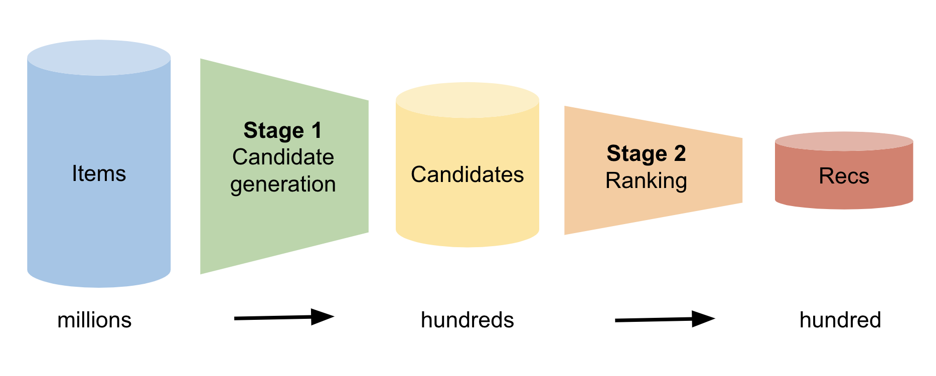 Figure 1. Flow of a two-stage candidate reranker recommendation system
Stage 1: Candidate generation
There are many ways to generate candidates, including statistical methods and deep learning methods. One statistical technique to generate candidates is building a co-visitation matrix. You iterate through all user historical sessions and maintain a cumulative tally of how often each pair of items coexists within user sessions. As a result, you know the top 100 items that are frequently paired with each item.
Now, given a specific user, you can generate candidate items by iterating through their user history and combining all top 100 lists associated with each item in their history. Many items appear multiple times. The candidates are the most common items in this concatenated list of hundreds of items.
Stage 2: Ranking
Using candidates from stage 1, build a tabular dataframe (Figure 2), which you use to train a reranker. Imagine that stage 1 produces 100 candidates per user. Then your tabular dataframe has 100 rows for each trained data user. One column is user and another column is candidate item. Add a third column for the target. Each row with a candidate item that is a correct match for that row’s user has a 1 in the target column and 0 otherwise.
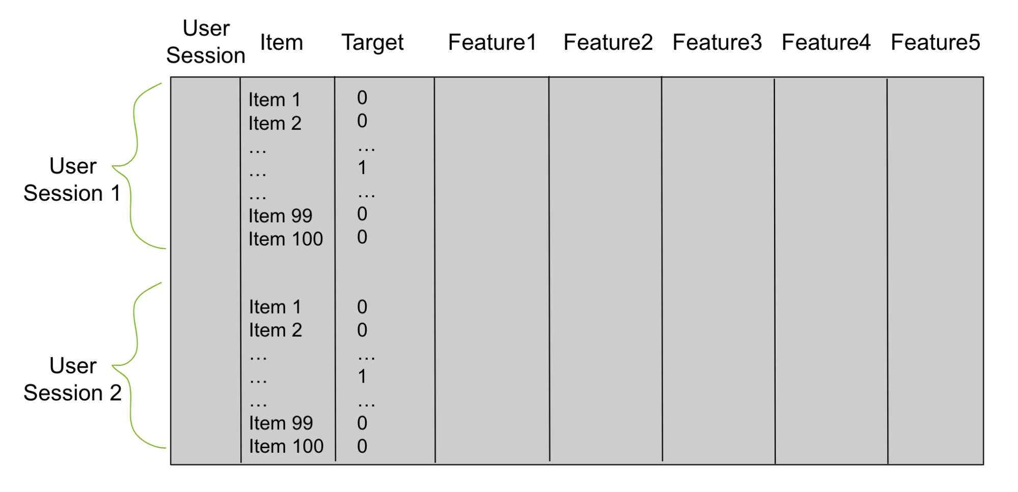 Figure 2. Reranker dataframe table
Next, add columns that describe the user sessions and items called feature columns. These feature columns are what the reranker uses to learn patterns and predict the target column. You train your reranker with either a binary classification objective or a pairwise or listwise ranking objective. Afterward, you use this trained model to predict items for unseen test user sessions.
Data scarcity in underrepresented languages
The two-stage candidate reranker approach (and any other approach) requires a large amount of training data to train the machine learning or deep learning model properly. Popular languages typically have lots of existing data, but this is not true for historically underrepresented languages.
Advocating for underserved languages is crucial for several reasons, such as promoting inclusivity, increasing global reach, and improving online user engagement and satisfaction.
To build recommender systems for underrepresented languages, I recommend using transfer learning. By leveraging datasets for common languages, models can recognize existing patterns and apply these learnings to support languages that are not widely spoken. This helps you overcome small dataset challenges and create a more inclusive digital world.
Pro tips for developing multilingual recommendation systems
To overcome data scarcity, use transfer learning to apply information from one language to another for stages 1 and 2. Many items have equivalents in multiple languages. Therefore, user-item interaction behavior in one language can be translated to another language.
Here are the top tips for speeding up the development process for multilingual recommendation engines.
Tips for candidate generation
- First, create co-visitation matrices for underrepresented languages by using user histories that exist in both popular languages and underrepresented languages.
- Be sure to represent items with pretrained multilingual large language model (LLM) embeddings. Then, use cosine similarity to find candidate items in underrepresented languages.
- Initialize NN embeddings with pretrained multilingual LLM embeddings. Then, fine-tune and use cosine similarity between user and item embeddings to find candidate items in the underrepresented languages.
Tips for ranking
- You can use item features from popular languages as item features for underrepresented languages in the tabular dataframe for the reranker.
- Create user-item interaction features by transferring user-item patterns learned from popular languages to underrepresented languages.
- Finally, train an underrepresented language’s reranker using user-item dataframe rows from popular languages.
Tutorial: Multilingual recommender system
To help you test these methods out, I walk you through an optimized process for building a multilingual recommender system.
Candidate generation implementation
The goal of candidate generation is to generate hundreds of item suggestions per user. Two popular techniques are using co-visitation matrices and using representation learning. Using transfer learning with co-visitation matrices is straightforward.
Earlier in this post, I discussed how co-visitation candidate generation is based on counting the coexisting pairs of product IDs within user histories. As many product IDs exist in multiple languages, you can use pairs from a German user’s history as counts in a Spanish co-visitation matrix. In Figure 3, the top German row is from the training data. You then “translate” it to Spanish, shown in the bottom row.
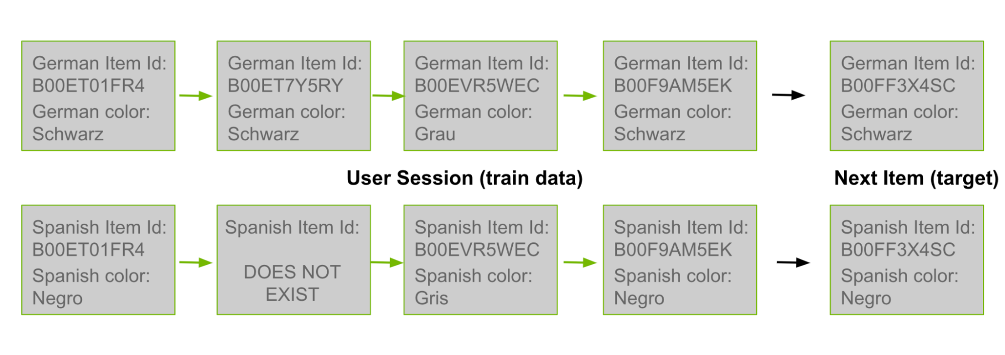 Figure 3. Transfer learning process
The procedure is as follows.
- Given a pair of Spanish product IDs, you can iterate through users from the other five languages: English, German, Japanese, Italian, and French.
- Whenever you observe the pair of Spanish product IDs in one of these user’s histories, add 1 to the count for this Spanish item pair. Or you can use a different weight, like adding 0.5 to the count.
- After you accumulate counts for all Spanish item pairs, continue to generate candidates as before by applying the new co-visitation matrix to each Spanish user’s history to generate candidates for the Spanish user.
The fastest and most efficient way to create co-visitation matrices is to use RAPIDS cuDF. To follow along, see the Candidate ReRank Model using Handcrafted Rules Jupyter notebook with example code.
By merging a dataframe that contains all user histories (that is, a dataframe with columns user and history item) to itself on the key user, you create all historical pairs. Then group by item pairs and aggregate the counts.
import cudf
df = cudf.DataFrame(ALL_USER_HISTORIES)
df = df.merge(df, on='user')
df['wgt'] = 1
df = df.groupby(['item_x','item_y']).wgt.sum()
Representation learning, LLMs, and deep learning embeddings are hot and current topics. Besides co-visitation matrices, an alternative to generating candidate items for each user is to create meaningful distance embeddings. If you have meaningful distance embeddings for each item, then you could use a model that predicts an embedding for each user. Next, find the 100 closest (through cosine similarity) embeddings to this predicted embedding and use these as your candidates (Figure 4).
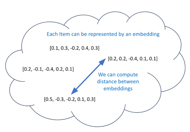 Figure 4. Compute distance between embeddings
The process of training meaningful distance embeddings for items is called representation learning. Embeddings are N dimensional vectors in N dimensional space. During training, embeddings of similar items are modified to be closer together (through some distance metric) while embeddings of dissimilar items are modified to have at least a predefined gap distance (margin) between them.
One way to use transfer learning during representation learning is to pre-initialize the embeddings with multilingual sentence embeddings. Each item has a title, whether it’s in English, German, Japan, Spanish, Italian, or French. You can pre-initialize each item with its title embedding from Hugging Face’s model stsb-xlm-r-multilingual, for example. This model has been trained on many different languages and transfers learning from all of them. Afterward, you can fine-tune the embeddings using your training data with the model shown in Figure 5.
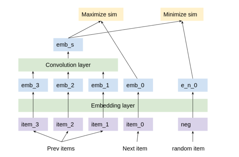 Figure 5. Representation learning
Fine-tune your model using all train data user histories. Every three consecutive history items are paired with one positive item target, which is the next consecutive item. Each triplet is paired with 4096 negative item targets, which are randomly chosen items. Backpropagation maximizes cosine similarity between the predicted embedding and positive target. And it minimizes cosine similarity between the predicted embedding and negative target. Afterward, you have meaningful distance embeddings for each item and a predicted embedding for each user.
A quick and easy way to create transformer-based, session-aware recommender systems that can use pretrained embeddings is to use the NVIDIA Merlin framework. For more information, see the Session-Based Next Item Prediction for Fashion E-Commerce and Training With Pretrained Embeddings Jupyter notebooks.
You can also feed your models with NVIDIA Merlin Dataloader.
Ranking implementation
The goal of stage 2 is to train a reranker that predicts the likelihood of each candidate item being correct among all possible candidate items for each user. To train a model successfully, you need feature columns in addition to a user, item, and target column. There are three types of feature columns:
- Item features
- User features
- User-item interaction features
 Figure 6. Reranker dataframe with features
Item features describe items. For example, you can add an item price feature. Then, every row in your reranker dataframe with item A has a corresponding price A in the item price column (Figure 6).
Using transfer learning on item features is easy. To transfer learning from German to Spanish, you can create item features from the German user history data and then merge it to Spanish items.
For example, for each item product ID, count how often it appears in all German user histories. Then every row in your reranker dataframe with Spanish item A has a corresponding German popularity A in the German item popularity column. The reason this works is because many item product IDs exist in both German and Spanish. If a certain Spanish product ID does not exist in German, then you insert NAN in the German item popularity column.
User feature columns and item feature columns are generally created with dataframe groupby commands. Create a property for each user or item and then merge it into your dataframe. The quickest and most efficient method is to use RAPIDS cuDF.
import cudf
item_features = data.groupby(‘item’)
.agg({‘item:count’,’user:nunique’,’price:first’})
df = df.merge(item_features, left_on=’item’,
   right_index=True, how=’left’)
user_features = data.groupby(‘user’)
.agg({‘user:count’,’item:nunique’})
df = df.merge(user_features, left_on=’user’,
   right_index=True, how=’left’)
User-item interaction features describe the relationship between a row’s candidate item and that row’s user. These features have a different value for each row. A common way to generate user-item interaction features is to describe the relationship between a user’s last history item and their candidate item.
One way to use transfer learning from popular languages to underrepresented languages is to create meaningful distance embeddings for all items using multilingual information. Then a user-item interaction feature can be the cosine similarity score between a user’s last history item and candidate item based on the embeddings.
Figure 7 shows extracting item embeddings from a multilingual LLM. You concatenate all the text for each item and input it into your LLM. Extract the last hidden layer activations as your embedding.
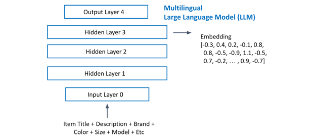 Figure 7. Large language model embeddings
A third way to use information from popular languages to improve underrepresented language recommendation is to train your underrepresented GBT reranker using dataframe rows from popular languages. First, you use the same column features for all language dataframes and then you merge all dataframes into one new dataframe. Afterward, your dataframe is large.
The best way to train GBT with millions of rows is to use RAPIDS Dask cuDF XGB, which uses multiple GPUs! For more information, see the KDD cup solution code.
The key lines of the code are as follows:
import xgboost as xgb
import dask, dask_cudf
from dask.distributed import Client
client = Client(cluster)
df = dask_cudf.read_parquet(FILES).persist()
dtrain = xgb.dask.DaskQuantileDMatrix(
client, df[FEATURES], df[TARGET])
xgb.dask.train(client, xgb_parms, dtrain)
Conclusion
When browsing online, recommendation systems may seem magical but, as you learned throughout this post, the inner workings of a multilingual recommendation engine are deterministic and understandable.
In this post, I shared techniques that the Kaggle Grandmasters of NVIDIA and NVIDIA Merlin teams used to win the recent KDD cup 2023 Multilingual Recommender System competition hosted by Amazon.
I also introduced the two-stage candidate reranker technique for recommendation systems. This is a powerful technique that helps solve many recommender system needs. Next, I gave you pro tips to help train recommendation systems for underrepresented languages. I shared how RAPIDS and NVIDIA Merlin frameworks can help you build recommender systems.
I hope that you can use some of these ideas in your next recommender system project. By improving online recommender systems for underrepresented languages, we can all make the Internet more inclusive, extend global reach, and improve user engagement and satisfaction.
Source:: NVIDIA