Recent years have seen a proliferation of large language models (LLMs) that extend beyond traditional language tasks to generative AI. This includes models like…
Recent years have seen a proliferation of large language models (LLMs) that extend beyond traditional language tasks to generative AI. This includes models like ChatGPT and Stable Diffusion. As this generative AI focus continues to grow, there is a rising need for a modern machine learning (ML) infrastructure that makes scalability accessible to the everyday practitioner.
This post presents how two open-source frameworks, Alpa.ai and Ray.io, work together to achieve the scale required to train a 175 billion-parameter JAX transformer model with pipeline parallelism. We provide a detailed exploration of these two integrated frameworks, as well as their combined architectures, developer-friendly API, scalability, and performance.
Both Alpa and Ray are, at the core, designed to enhance developer velocity and scale models efficiently. The pipeline parallelism feature of the Alpa framework easily parallelizes the computation of large models across multiple GPUs and offloads the cognitive burden from the developer. Ray offers a distributed computing framework that enables simplified scaling and management of resources across multiple machines.
When used together, Alpa and Ray offer a scalable and efficient solution to train LLMs across large GPU clusters. With this integration, the benchmarks show the following benefits:
Overview of large language models
Large language models (LLMs) are primarily based on transformer architecture. The seminal 2017 paper, Attention Is All You Need, spurred myriad variations of transformer-based models, increasing exponentially in billions of training parameters. These variations—such as BERT, RoBERTa, GPT-2 and GPT-3, and ChatGPT—were all styled on transformers that incorporate the core architectural components of multihead attention and encoder/decoder block.
Due to intense research in academia and across industries, a rapid release of models with training parameters in the billions ensued over a short period. Complemented by the recent Diffusion and DALL-E language models, LLMs introduce the notion of generative AI: the ability to feed the model different input modalities—text, video, audio, and images—to analyze, synthesize, and generate new content as simple sequence-to-sequence tasks.
Generative AI is the next era in natural language processing (NLP). To learn more, see What Is Generative AI? and What’s the Big Deal with Generative AI? Is it the Future or the Present?
Unique challenges come with training these billion-parameter LLM models from scratch or fine-tuning them with new data. To train and evaluate LLM models demands massive distributed computing power, clusters of accelerated-based hardware and memory, reliable and scalable machine learning frameworks, and fault-tolerant systems. In the following sections, we discuss these challenges and offer our approach to addressing them.
Machine learning system challenges of LLMs
The parameter size of a modern LLM is at the magnitude of hundreds of billions, which exceeds the GPU memory of a single device or host. For example, an OPT-175B model requires GPU memory of 350 GB just to accommodate the model parameters—not to mention the GPU memory needed for gradients and optimizer states during training, which can push memory requirements beyond 1 TB. To learn more, see Democratizing Access to Large-Scale Language Models with OPT-175B.
Meanwhile, commodity GPUs only have 16 GB / 24 GB GPU memory, and even the most advanced NVIDIA A100 and H100 GPUs only have 40 GB / 80 GB of GPU memory per device.
To run training and inference for LLMs efficiently, developers need to partition the model across its computation graph, parameters, and optimizer states, such that each partition fits within the memory limit of a single GPU host. Based on the GPU cluster available, ML researchers must adhere to a strategy that optimizes across different parallelization dimensions to enable efficient training.
Currently, however, optimizing training across different parallelization dimensions (data, model, and pipeline) is a difficult, manual process. Existing dimensional partition strategies of an LLM include the following categories:
- Interoperator parallelism: Partition the full computation graph to disjoint subgraphs. Each device computes its assigned subgraph and communicates with other devices upon finishing.
- Intraoperator parallelism: Partition matrices participate in the operator to submatrices. Each device computes its assigned submatrices and communicates with other devices when multiplication or addition takes place.
- Combined: Both strategies can be applied to the same computation graph.
Note that some research work categorizes model parallelism as ‘3D parallelism’ that represents data, tensor, and pipeline parallelism, respectively. In Alpa’s terminology, data is simply the outer dimension of tensor parallelism that maps to intraoperator parallelism, and pipeline parallelism is the result of interoperator parallelism that partitions a graph into separate stages with pipelining orchestration. These are equivalent in power, so we will keep the partitioning terminology simple and consistent, using the terms ‘interoperator’ and ‘intraoperator’ parallelism for the remainder of the post.
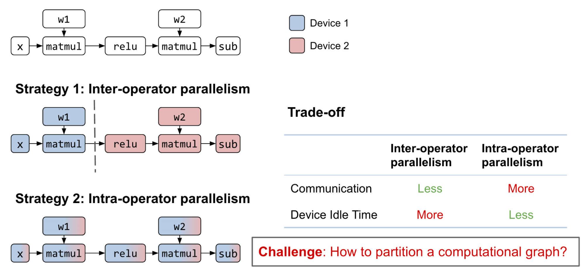 Figure 1. Partition strategies for interoperator and intraoperator parallelism
Exploring the possible strategies of interoperator and intraoperator parallelism is a challenging combinatorial problem with various tradeoffs. With reasonable computation graph partitioning of interoperator parallelism, the communication cost can be small between subgraphs, but introduces data dependency. Although pipelining can help alleviate the problem, device idle time is still inevitable.
On the other hand, intraoperator parallelism can parallelize the operator computation among multiple GPU devices with less idle time when the next operator cannot preserve matrix partition from the previous one. This approach comes with a higher communication cost.
In addition to partitioning matrices and computation graphs, the ability to map partitions to GPU devices with awareness of the heterogeneous network topology is needed. GPU connections inside a node (NVIDIA NVLink) are orders of magnitude faster than interhost networking (InfiniBand, EFA, Ethernet), and will lead to significant performance differences among different partition strategies.
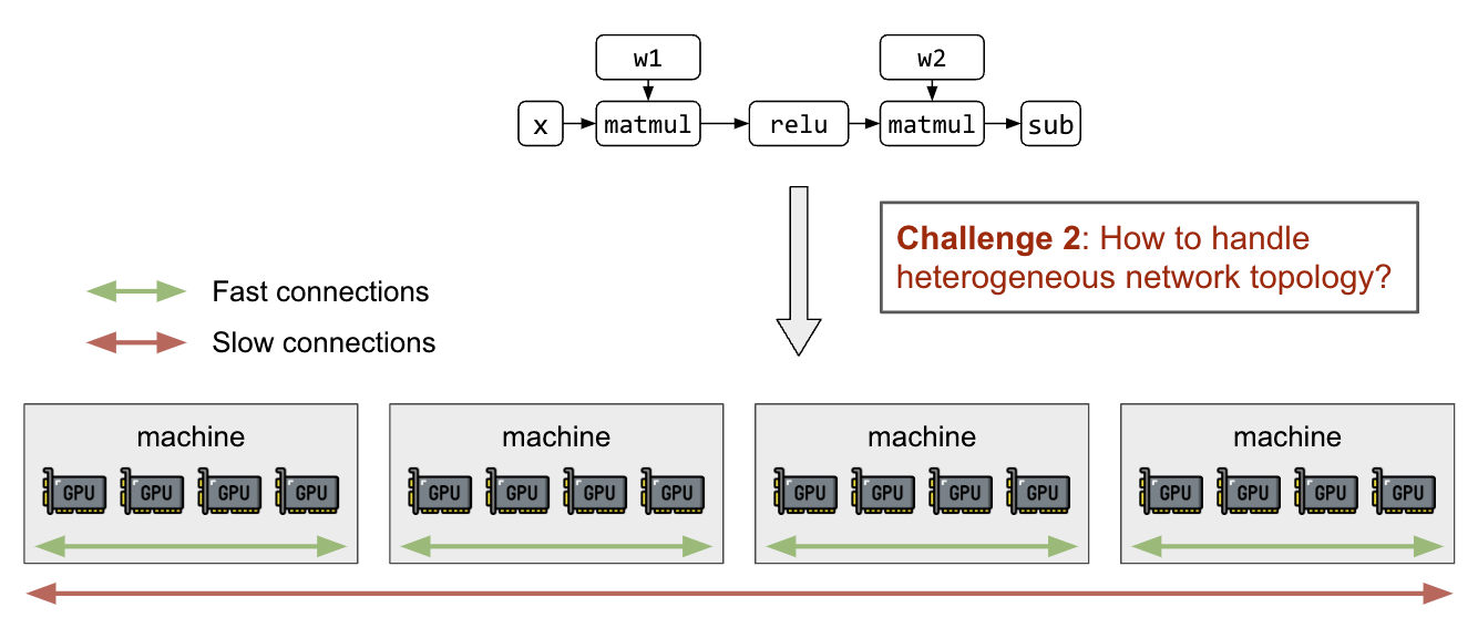 Figure 2. Network topology of GPU clusters
Prior LLM partitioning work
Prior work in the model parallelism domain has achieved different parallelism techniques (Figure 3). As explained above, determining and executing an optimal model partitioning strategy is a manual process that requires deep domain expertise.
Alpa handles interoperator and intraoperator parallelism automatically with a one-line decorator. This seamlessly devises a partition strategy for data, tensor, and pipeline parallelism for LLMs at scale. Alpa is also capable of generalizing to a wide range of model architectures, which greatly simplifies model parallelism to make LLMs more accessible to everyone.
Architecture overview
Before describing the solution to these challenges using our layered technical stack, it is important to provide an architectural overview of the stack’s critical components (Figure 3). These components include a GPU accelerator at the base, followed by a compilation and runtime layer, GPU management and orchestration, automatic model parallelization (Alpa), and, finally, model definition at the top.
 Figure 3. Technical integration layered stack for LLMs
Introduction to Alpa
Alpa is a unified compiler that automatically discovers and executes the best interoperator and intraoperator parallelism for large deep learning models.
Alpa’s key API is a simple @alpa.parallelize decorator that parallelizes and optimizes for the best model parallelism strategy automatically. Given the JAX static graph definition with known sizes and shapes, a simple tracing on the train_step with a sample batch is sufficient to capture all the information required for automatic partitioning and parallelization. Consider the simple code below:
@alpa.parallelize
def train_step(model_state, batch):
    def loss_func(params):
        out = model_state.forward(params, batch["x"])
        return np.mean((out - batch["y"]) ** 2)

    grads = grad(loss_func)(state.params)
    new_model_state = model_state.apply_gradient(grads)
    return new_model_state

# A typical JAX training loop
model_state = create_train_state()
for batch in data_loader:
    model_state = train_step(model_state, batch)
Automatic parallelization passes in Alpa
Alpa introduces a unique approach to tackling the complex parallel strategy search space of a two-level hierarchical system. Traditional methods have struggled to find a unified algorithm that derives an optimal parallel strategy from the vast space of interoperator and intraoperator options. Alpa addresses this challenge by decoupling and reorganizing the search space at different levels.
At the first level, Alpa searches for the most effective interoperator parallel plan. Then, at the second level, the best intraoperator parallel plan for each stage of the interoperator parallel plan is derived.
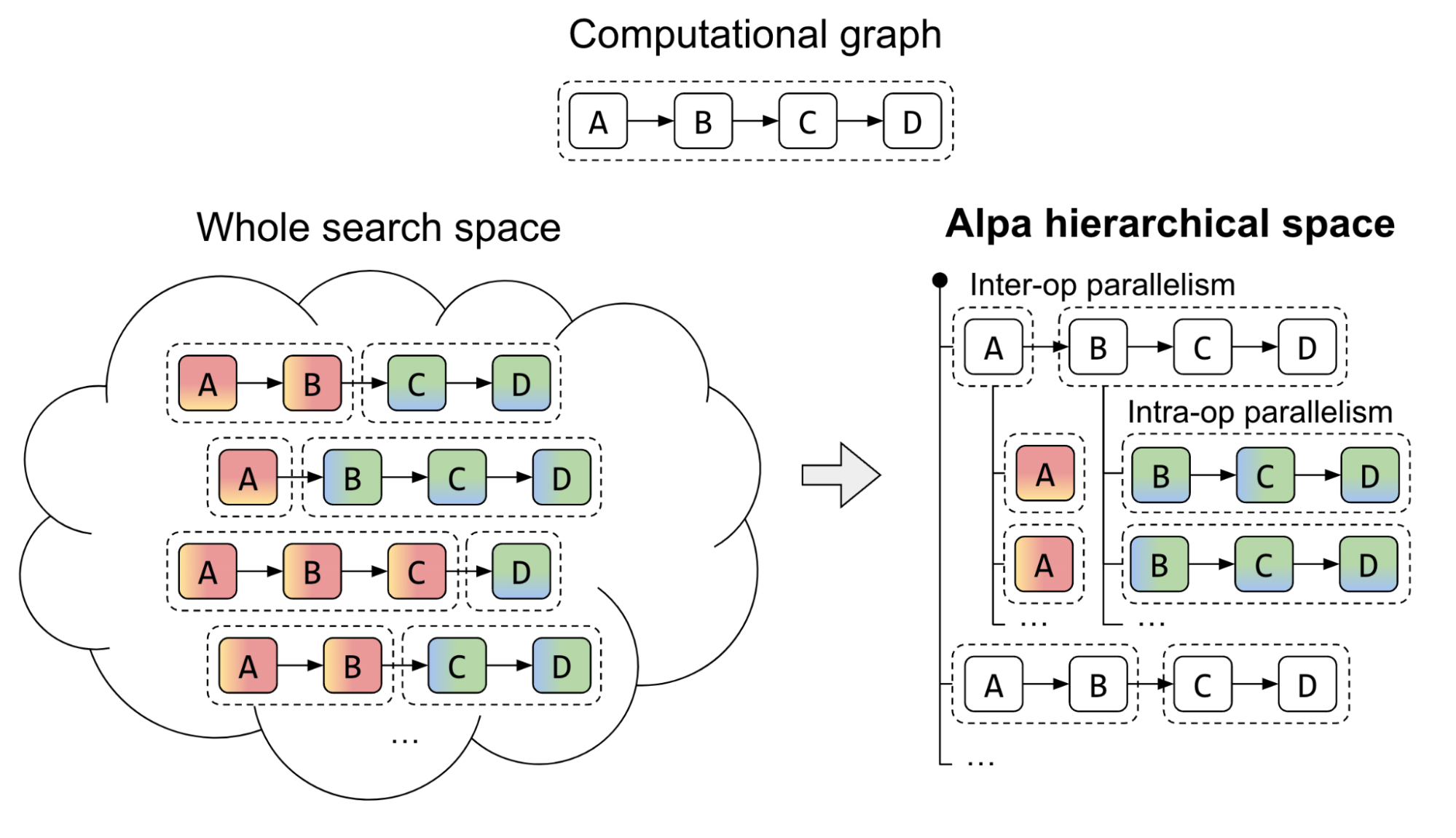 Figure 4. The Alpa hierarchical search space for partitioning strategy
The Alpa compiler is built around the search space decomposition approach introduced previously. Its input consists of a computational graph and a cluster specification. To optimize the parallel strategy, Alpa conducts two compiler passes:
- First pass: Interoperator uses dynamic programming to identify the most suitable interoperator parallelism strategy.
- Second pass: Intraoperator uses integer linear programming to identify the best intraoperator parallelism strategy.
The optimization process is hierarchical. The higher-level interoperator pass calls the lower-level intraoperator pass multiple times, making decisions based on the feedback from the intraoperator pass. Then, the runtime orchestration pass executes the parallel plan and brings the strategy to life.
In the next section, we discuss Ray, the distributed programming framework on which Alpa is built. This will show how GPU cluster virtualization and pipeline parallelism runtime orchestration are enabled to empower LLMs at scale.
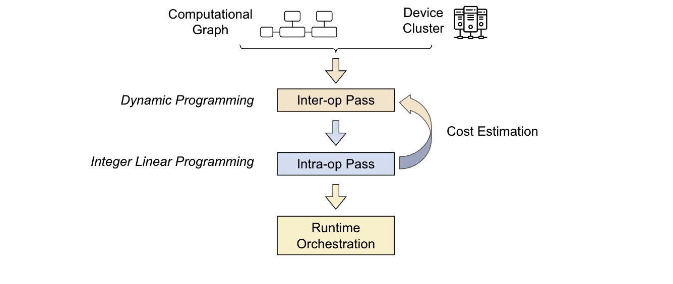 Figure 5. Alpa automatic partitioning passes at different levels
Introduction to Ray
Ray is a general-purpose unified framework for scaling and simplifying ML compute. For the purposes of this discussion, there are two key Ray primitives that you should be aware of: tasks and actors.
Ray task
A Ray task is stateless and is as simple as a function when decorated with @ray.remote. A Ray task can be dispatched to execute anywhere in a cluster of machines. Invocations, through f.remote(args), are executed in parallel and are asynchronous in nature. They return a future object reference, the value of which is retrieved using ray.get(object_ref).
 Figure 6. A Ray task is a stateless Python simple function
Ray actor
A Ray actor is a Python class that is stateful. It is a fundamental building block in Ray that enables a class to be remotely executed in a cluster, maintaining its state. Leveraging a Ray actor on a multitude of GPU devices enables access to various compelling capabilities.
For instance, when dealing with a stateful class, developers can run a preferred client like XLA runtime or HTTP. XLA is the compiler for linear algebra that empowers both JAX and TensorFlow under the hood. The XLA runtime client enables optimizing the model graph and automatically fuses individual operators.
Using Ray patterns and primitives as advanced abstractions
With these simple Ray primitives, such as Ray tasks and actors, it is possible to formulate a few simple patterns. The following sections will uncover how these primitives can be used to build advanced abstractions—such as DeviceMesh, GPU Buffer, and Ray Collective—to empower LLMs at scale.
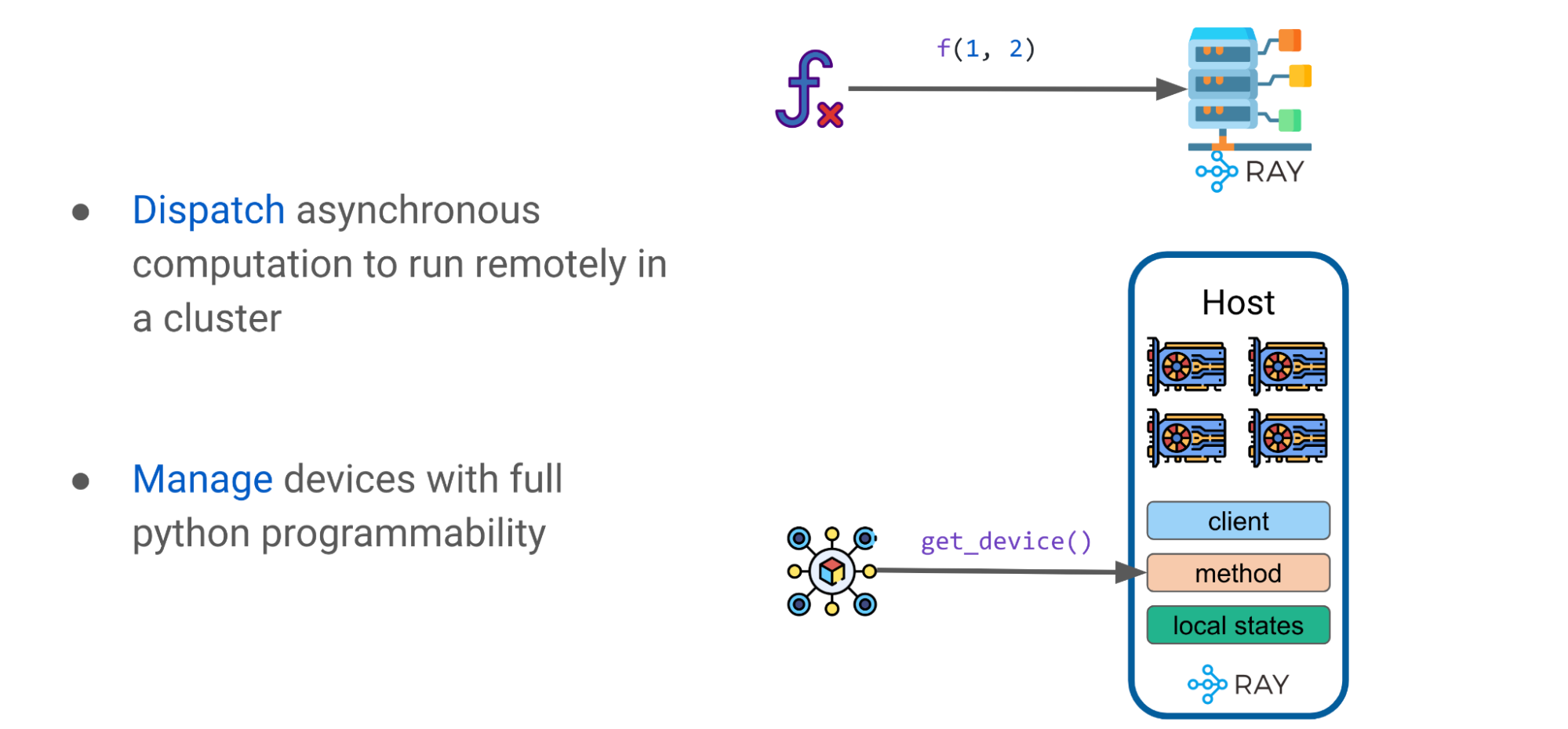 Figure 7. Ray patterns with tasks and actors
Advanced pattern: DeviceMesh
As explained previously, efficiently scaling LLMs requires partition model weights and computations on multiple GPU devices. Alpa uses Ray actors to create more advanced device management abstractions such as DeviceMesh, a two-dimensional mesh of GPU devices (Figure 8).
A logical mesh can span multiple physical hosts, including all their GPU devices, with each mesh acquiring a slice of all GPUs on the same host. Multiple meshes can reside on the same host, and a mesh can even encompass an entire host. Ray actors offer tremendous flexibility in managing GPU devices within a cluster.
For example, you can choose to have one actor per host, one per mesh, or one per device, depending on the level of orchestration control you require.
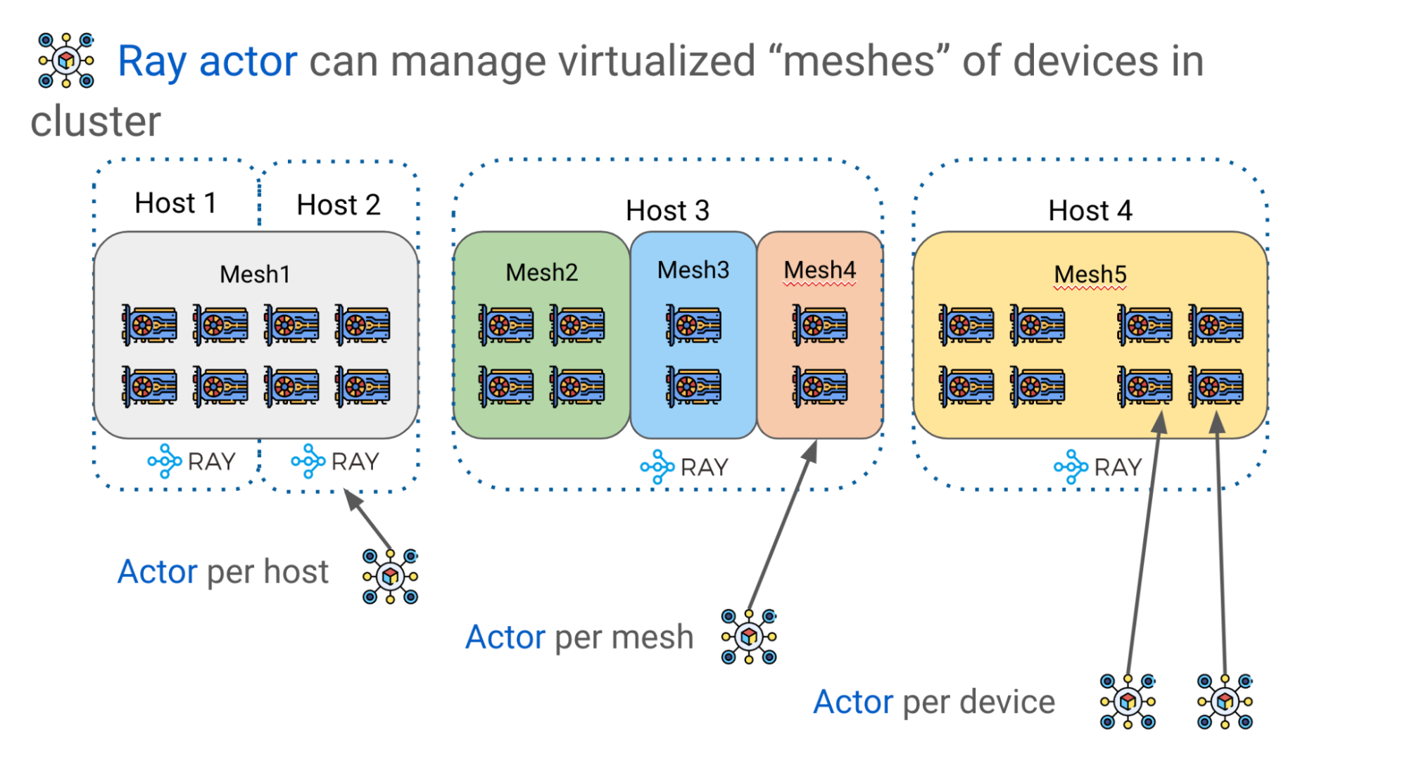 Figure 8. DeviceMesh managed by Ray actors for GPU cluster virtualization and management
Advanced pattern: GPU buffer
The second advanced pattern in Alpa is GPU buffer management across DeviceMeshes. GPU computations often result in GPU tensors that represent tiles of a larger matrix. Alpa has an application-level GPU buffer management system that assigns a UUID for each GPU buffer and provides basic primitives, such as Send/Recv/Delete, to enable cross-mesh tensor movement and lifecycle management.
Using a Ray actor and DeviceMesh abstractions, buffers can be managed and transferred by invoking corresponding methods on the host to facilitate advanced model training paradigms.
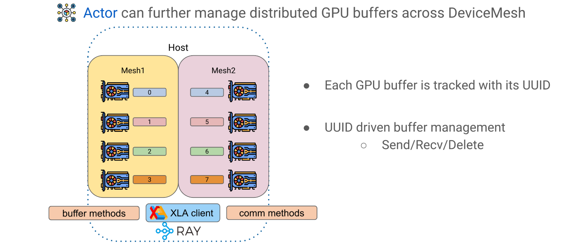 Figure 9. GPU buffer management with a Ray actor
Advanced pattern: Ray collective communication library
The third advanced pattern is the Ray collective communication library, a collection of communication primitives that enables efficient and flexible tensor movement across different CPUs, GPUs, and DeviceMeshes. It is an essential communication layer for pipeline parallelism.
The simple intrahost case is depicted on the left side of Figure 10 (Host 1), where GPU devices are interconnected with NVlink. The right side of Figure 10 (Hosts 2 and 3) shows the multimesh, multihost scenario, where communication occurs in a potentially more heterogeneous setup with a mix of intrahost NVLink and interhost networking (InfiniBand, EFA, or Ethernet).
Using the Ray collective communication library, you can move and reshard tensors freely across DeviceMeshes through high-performance networking with the NVIDIA Collective Communications Library (NCCL).
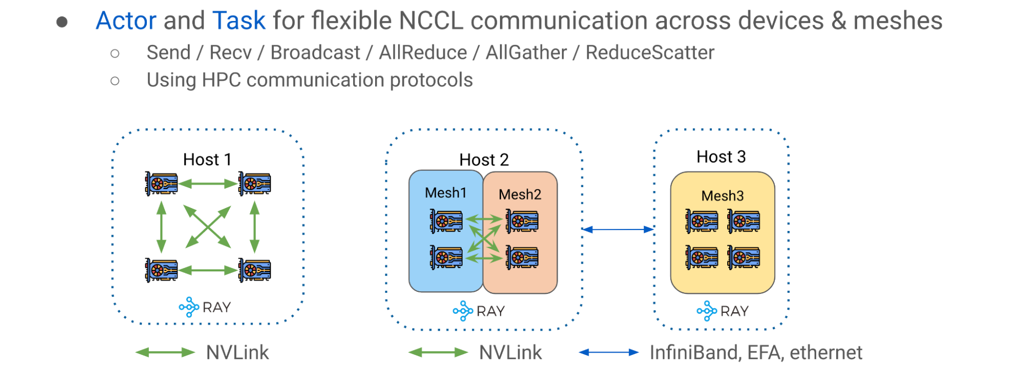 Figure 10. Ray collective communication for cross mesh tensor movement through NCCL
Pipeline parallelism runtime orchestration
In JAX and Alpa, computations, communication, and instructions are often created to be static. The static artifact is an important property, because in JAX a user program can be compiled to intermediate representations (IR) and then fed to XLA as a self-contained executable. Users can pass inputs into the executable and expect results as outputs where all tensors are known in size and shape, just like a function for tensors.
The end-to-end flow can be roughly divided into the following stages:
- Each instruction is a self-contained JAX HLO/XLA program that can be of type RUN, SEND, RECV, or FREE. Each can allocate, transfer, or free the GPU buffer across DeviceMesh(es).
- Static instructions greatly reduced scheduling frequency and overhead at the Ray single-controller level for better performance and scalability.
- Put compiled executables into corresponding host Ray actors for later invocation.
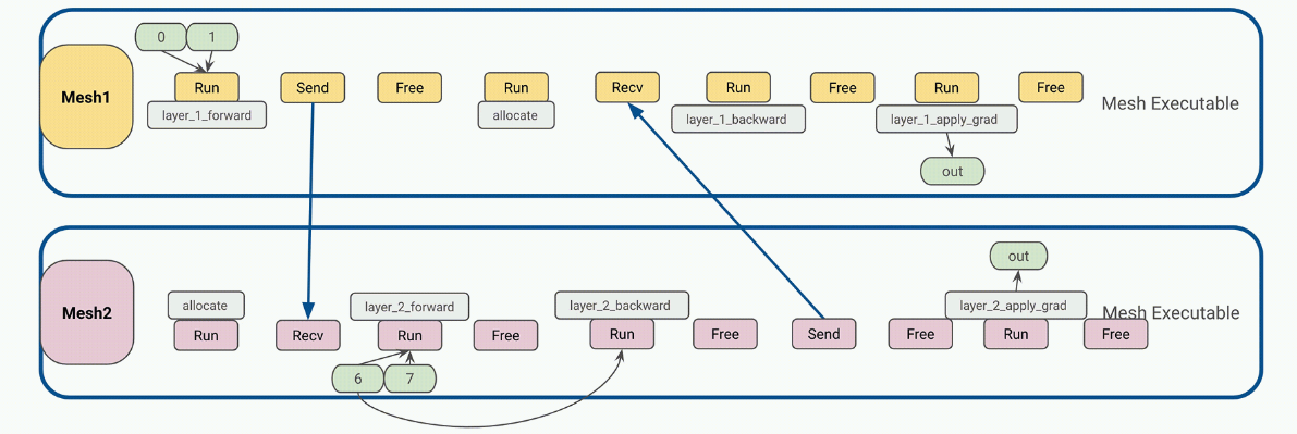 Figure 11. Example static instruction for two-layer pipeline parallelism
4. Driver calls and orchestrates compiled executables on each host worker to begin end-to-end pipelined transformer training.
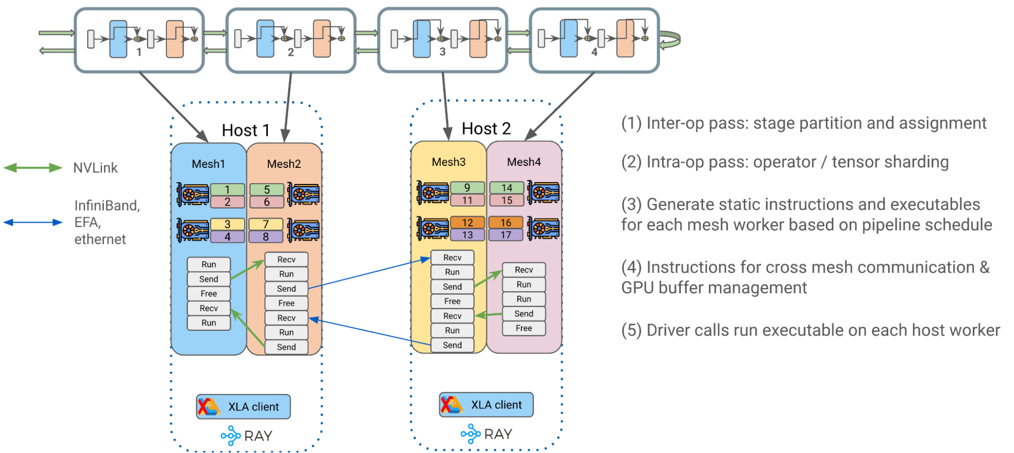 Figure 12. End-to-end pipeline parallelism runtime orchestration with Alpa on Ray
Alpa on Ray benchmark results
We closely collaborated with NVIDIA to benchmark this effort for accurate performance and scalability results. For scalability and performance, the charts below, verified on an NVIDIA Selene cluster, demonstrate total HW FLOPs throughput of OPT-175B. Various GPU cluster sizes are used with peak HW FLOPs utilization of ~57.5% at ~179 TFLOPs per GPU. Model parallelization and partitioning are done automatically with a one-line decorator.
These benchmark results strongly suggest that Alpa on Ray is one of the most performant and scalable frameworks for training LLM models in JAX, even at a scale of 175 billion. Furthermore, Alpa on Ray is capable of finding and executing optimal parallelization strategies automatically.
Figure 13 provides more details about the model definition and other configurations used to achieve the results.
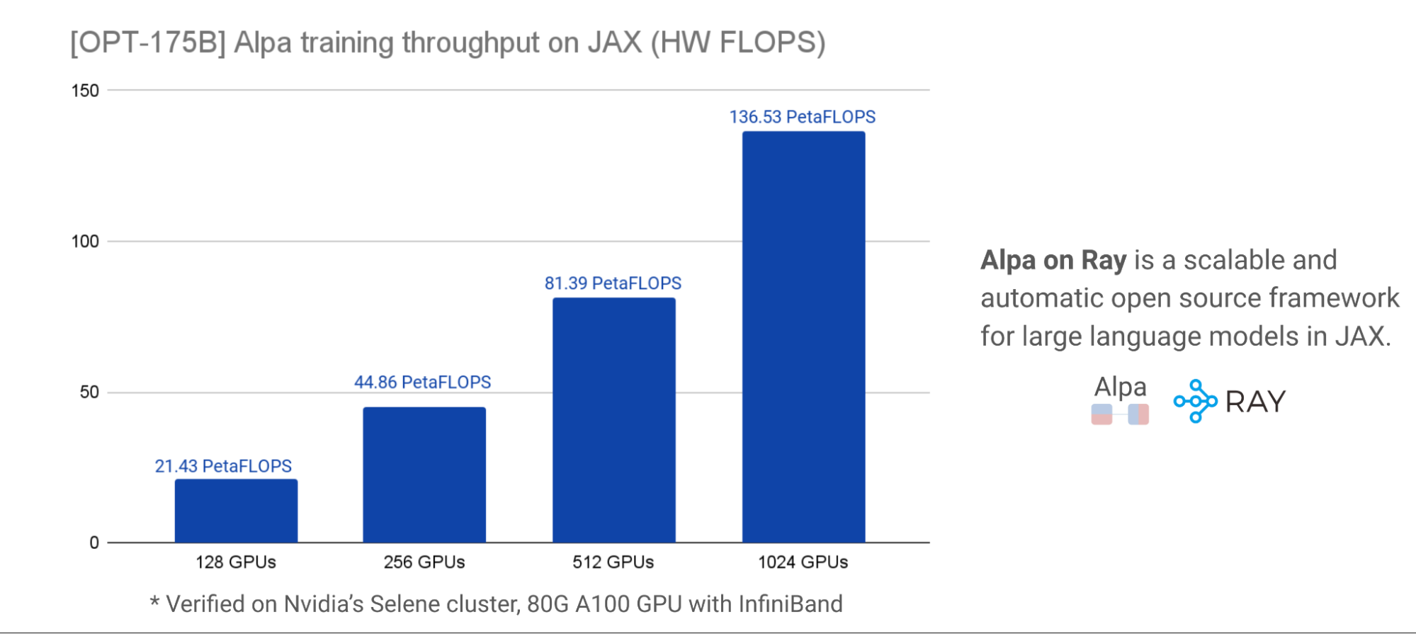 Figure 13. OPT-175B training throughput with Alpa on Ray, HW FLOPS
Summary
Combining Alpa and Ray OSS frameworks, developers can efficiently scale LLM training across a large cluster on JAX. Use Alpa to automatically compile your network architecture, and use Ray to orchestrate and run your tasks across a cluster of machines.
Our team estimates the addition of the following capabilities to enable users with greater performance and flexibility:
- Support for T5 with bf16 + pipeline parallelism at larger scale. We have enabled and benchmarked at four-host scale within capacity constraints.
- Further simplified LLM accessibility on commodity GPUs.
Additional resources
Want more information about Ray, Ray AIR, and Ray on Alpa?
- Learn How Ray Solves Common Production Challenges for Generative AI Infrastructure.
- Check out Ray on GitHub for sources and more.
- Explore the Ray documentation.
- Join the monthly Ray Meetup to discuss all things Ray.
- Connect with the Ray community.
- Register for Ray Summit 2023.
Want more information about Alpa?
- Check out Alpa on GitHub for the latest examples of LLM training and inference.
- Connect with the Alpa community on Slack.
Acknowledgements
Our team thanks AWS and CoreWeave for their generous support and sponsorship of our work on NVIDIA A100 Tensor Core GPUs to facilitate our interactive development. We also thank NVIDIA for internal NVIDIA Selene cluster access for benchmarking at scale and partnering with us throughout this collaboration.
Source:: NVIDIA
