
GPUs continue to get faster with each new generation, and it is often the case that each activity on the GPU (such as a kernel or memory copy) completes very…
GPUs continue to get faster with each new generation, and it is often the case that each activity on the GPU (such as a kernel or memory copy) completes very quickly. In the past, each activity had to be separately scheduled (launched) by the CPU, and associated overheads could accumulate to become a performance bottleneck. The CUDA Graphs facility addresses this problem by enabling multiple GPU activities to be scheduled as a single computational graph.
This post describes how CUDA Graphs have been recently leveraged by GROMACS, a simulation package for biomolecular systems and one of the most highly used scientific software applications worldwide. We will introduce CUDA Graphs and GROMACS, describe our work to integrate CUDA Graphs into (and co-design with) GROMACS, present performance results, and show you how to use CUDA Graphs within GROMACS.
GROMACS has evolved, over a multiyear collaboration between NVIDIA and the core GROMACS developers, to take full advantage of modern GPU-accelerated servers. For more details, see Creating Faster Molecular Dynamics Simulations with GROMACS 2020, Maximizing GROMACS Throughput with Multiple Simulations per GPU Using MPS and MIG, Massively Improved Multi-node NVIDIA GPU Scalability with GROMACS, and Heterogeneous parallelization and acceleration of molecular dynamics simulations in GROMACS (and references therein).
Background
The latest step on the GROMACS journey is to use CUDA Graphs to further enhance performance. This feature is available in the new 2023 release. This co-design effort includes not only application-level experts, but also the NVIDIA CUDA software development team. Improving GROMACS in unison with the cutting-edge CUDA Graphs technology will ultimately benefit other applications.
CUDA Graphs
This section provides a very brief overview of CUDA Graphs, structured in a GROMACS-friendly way. See the previous post, Getting Started with CUDA Graphs, for a thorough introduction to CUDA Graphs.
Figure 1 depicts the scheduling and execution of a number of GPU activities. With the traditional stream model (left), each GPU activity is scheduled separately by a CPU API call. Using CUDA Graphs (right), a single API call can schedule the full set of GPU activities.
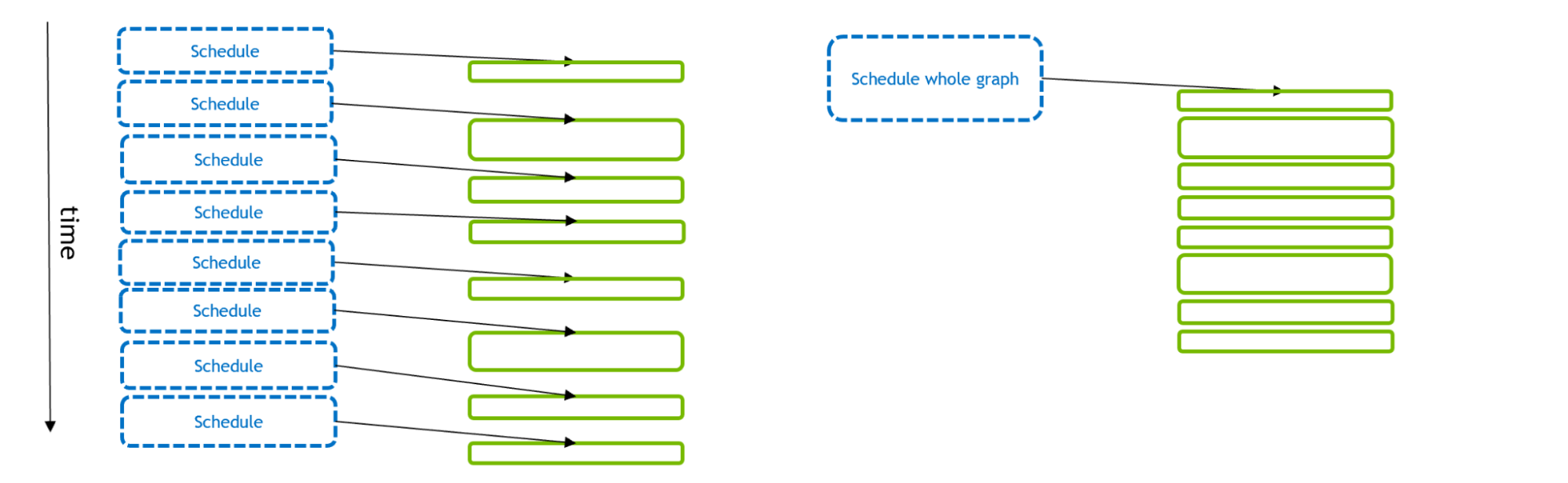 Figure 1. An illustration of the time taken to schedule and execute GPU activities, with the traditional stream model on the left and CUDA Graphs model on the right. GPU activity is indicated by solid green rectangles and CPU API calls are indicated by blue rectangles.
If the GPU activities are small, then it can take more time to schedule than to execute. This starves the GPU (leaving gaps between kernels), with suboptimal overall execution. But if multiple-GPU activities are scheduled in a single CUDA graph, the CPU API time can be reduced, enabling more optimal GPU execution. In addition, with Graphs the CUDA driver has extra information about the workflow that it can exploit to optimize GPU execution of the graph itself.
As described in Getting Started with CUDA Graphs, it is relatively straightforward to adapt an existing stream-based code to use graphs. The functionality “captures” the stream execution into a graph, through a few extra CUDA API calls. We exploit this facility to enable the pre-existing GROMACS code to be executed using graphs instead of streams.
GROMACS
GROMACS is a key tool in understanding important biological processes, including those underlying pandemics such as COVID-19. Each GROMACS simulation evolves systems of many particles using the Newtonian equations of motion through repeated updates, where interparticle forces dictate particle movement.
Although the physics is fairly straightforward, the implementation is (necessarily) extremely complex to achieve very high performance, through multiple levels of parallelization and acceleration. As such, each simulation timestep involves a highly complex schedule of (often microsecond-scale) tasks.
Figure 2 shows, from left to right, how GROMACS has evolved to become an asynchronous GPU engine for molecular dynamics.
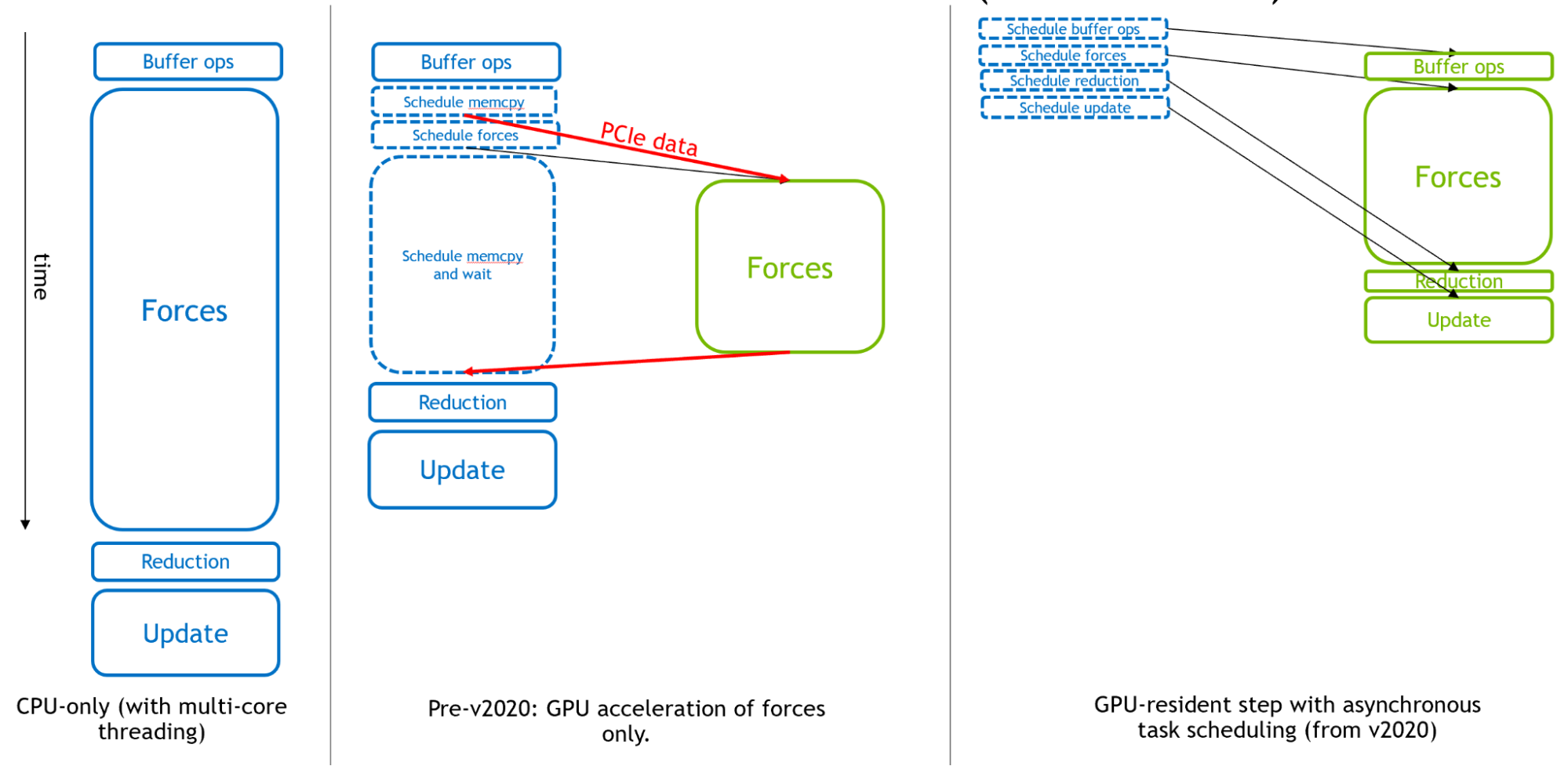 Figure 2. An illustration of the execution of GROMACS simulation timestep. In CPU-only mode (left), solid rectangles correspond to CPU calculations. With only forces offloaded to GPU (center), the CPU performs a mixture of calculations and scheduling activities. In the new GPU-resident mode (right), the CPU is only responsible for scheduling and all calculations are executed on GPU.
Originally, the CPU was used for the entirety of each simulation timestep. Then, in the early days of GPU computing, the expensive force calculations were offloaded to GPUs for effective overall acceleration.
Finally, in support of extremely fast modern GPUs, from GROMACS version 2020, all other components could be offloaded to enable a ‘GPU resident mode,’ where the simulation state remains on the GPU for multiple iterations, and the CPU is mainly responsible for scheduling activities executed asynchronously on the GPU. To learn more, see Creating Faster Molecular Dynamics Simulations with GROMACS 2020.
The right portion of Figure 2 shows how the GPU calculations, provided they are large enough, will form the “critical path” of execution, such that the performance of these components determine the overall simulation performance.
However, with ever-increasing GPU performance, small cases can be limited by CPU scheduling overhead rather than GPU execution, as described in the previous section. This is especially true when multiple GPUs are used in parallel to execute a single GROMACS simulation.
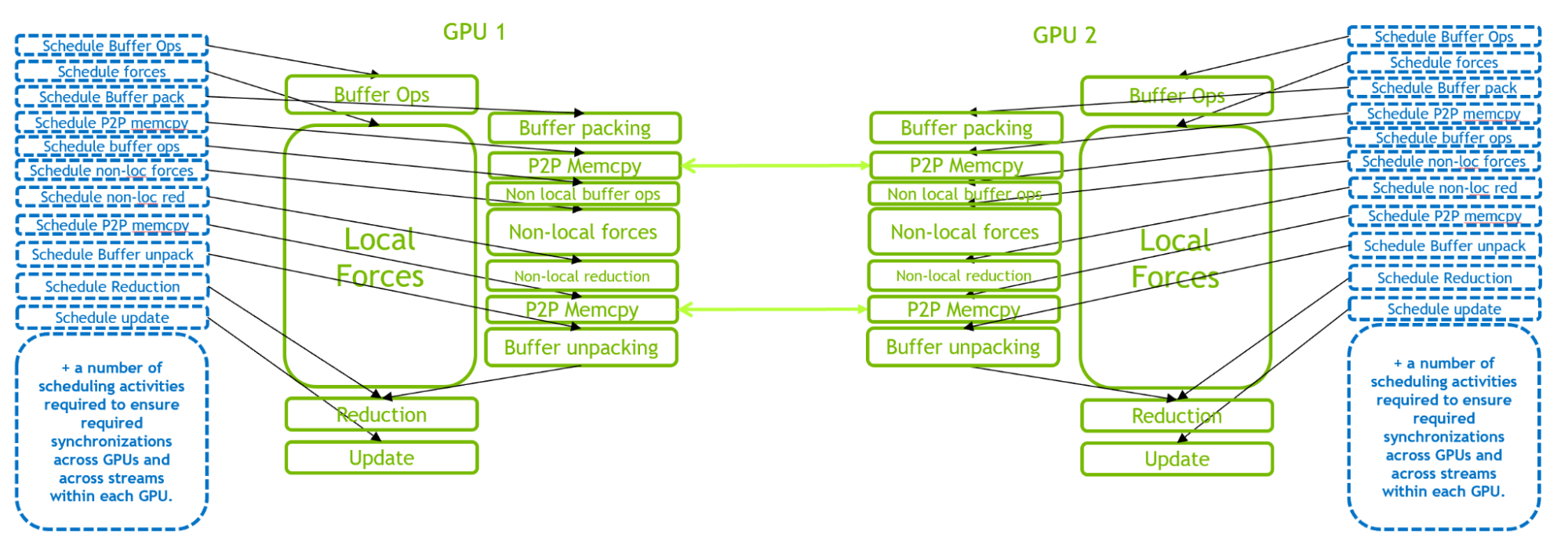 Figure 3. An illustration of the execution of GROMACS simulation timestep, for 2-GPU run. A much larger number of CPU scheduling activities exist to manage the multi-GPU communications and synchronizations.
Figure 3 illustrates the GPU-resident mode for a 2-GPU case. This scenario comes with a much more demanding CPU scheduling workload, compared to the single-GPU case, due to the complex intra- and inter-GPU interactions. The scheduling workload is even more demanding when more GPUs are introduced.
Hence, in many small cases, the performance bottleneck is CPU scheduling overhead rather than GPU execution. This has motivated the introduction of CUDA Graphs into GROMACS to enable multiple activities to be scheduled as a single graph, as described in the following section.
Implementing CUDA Graphs in GROMACS
This section describes the introduction of CUDA Graphs into GROMACS. At a high level, graph capture and replay functionality are used in a similar style to the example provided in Getting Started with CUDA Graphs.
There are a number of complexities in the GROMACS implementation related to the different types of tasks that GROMACS can perform on different steps, and complexities associated with managing the multi-GPU task and domain decomposition. Read on for a brief overview. For full technical details, see the GitLab Issue, Implement CUDA Graph Functionality and Perform Associated Refactoring, and the merge requests linked therein.
Note that GROMACS performs different types of simulation steps: “regular” steps plus infrequent “irregular” steps that include extra activities that must be performed once in a while (pressure coupling, temperature coupling, neighbor list update, domain decomposition, and many others). We have introduced CUDA Graphs into GROMACS by using a separate graph per step, and so-far only support regular steps which are fully GPU resident in nature.
On each simulation timestep:
- Check if this step can support CUDA Graphs. If yes:
- Check if a suitable graph already exists. If yes:
- Execute that graph
- Else: capture, instantiate, and save a new graph
- Check if a suitable graph already exists. If yes:
- Else: execute step using traditional streams
This enables execution using a CUDA Graph for the vast majority of steps. It is necessary to recapture and create a new graph executable for every neighbor-list or domain decomposition step (typically every 100-400 steps), which is infrequent enough to have minimal overhead.
For multi-GPU, use a single graph across all GPUs. So far, this is only supported with thread-MPI, where the multi-GPU graph is defined by exploiting the natural ability of CUDA to fork and join streams across different GPUs within the same process (using event-based GPU-side synchronization) and to automatically capture such workflows into a single graph.
We have created a new class in GROMACS to manage all the required functionality. For multi-GPU, this includes extra event-based fork and join operations to enable a single graph to be defined and executed across multiple GPUs.
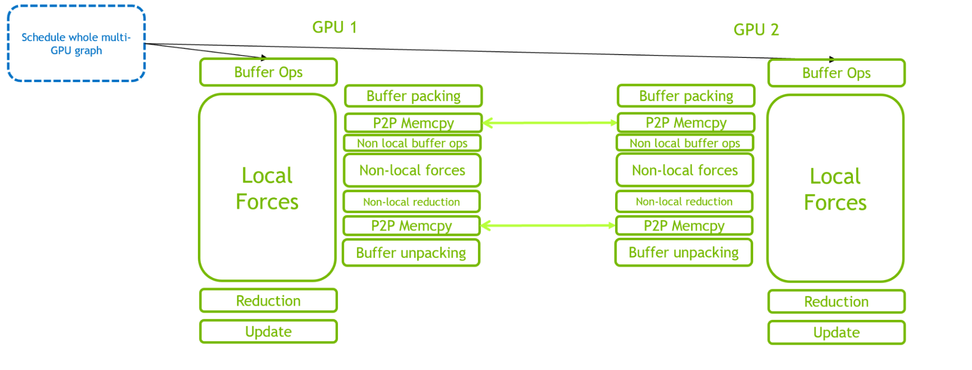 Figure 4. An illustration of the execution of GROMACS simulation timestep for 2-GPU run, where a single CUDA graph is used to schedule the full multi-GPU timestep
The benefits of CUDA Graphs in reducing CPU-side overhead are clear by comparing Figures 3 and 4. The critical path is shifted from CPU scheduling overhead to GPU computation.
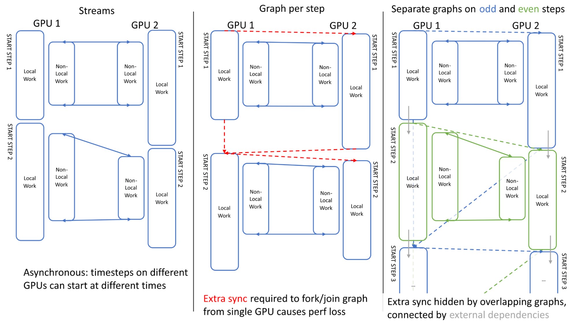 Figure 5. A comparison of stream and graph execution of two simulation timesteps on two GPUs
In order to maximize multi-GPU performance, it is important to ensure asynchrony across GPUs when linking multiple simulation timesteps. Figure 5 illustrates the GPU activities across two steps. It can be seen that, when using traditional streams, the execution is asynchronous across GPUs: GPU1 can start the second step before GPU 2 finishes its first step (left).
Our first attempt at scheduling using a single graph encountered an issue: the extra synchronization required to define the graph (forking/joining to start/end points on a single GPU) lost this asynchrony, causing overhead (center).
We overcame this problem by using a separate graph on odd and even steps (right), where these are linked using “external” CUDA events which can be recorded within one graph and enqueued within another (depicted by grey arrows), effectively overlapping the extra synchronization.
Figure 6 shows a real graph resulting from a regular timestep for a typical 4-GPU configuration. We do not intend to describe the details, but include this graph to provide a visual of the many activities and dependencies involved, and how CUDA Graphs is able to handle this complexity so effectively.
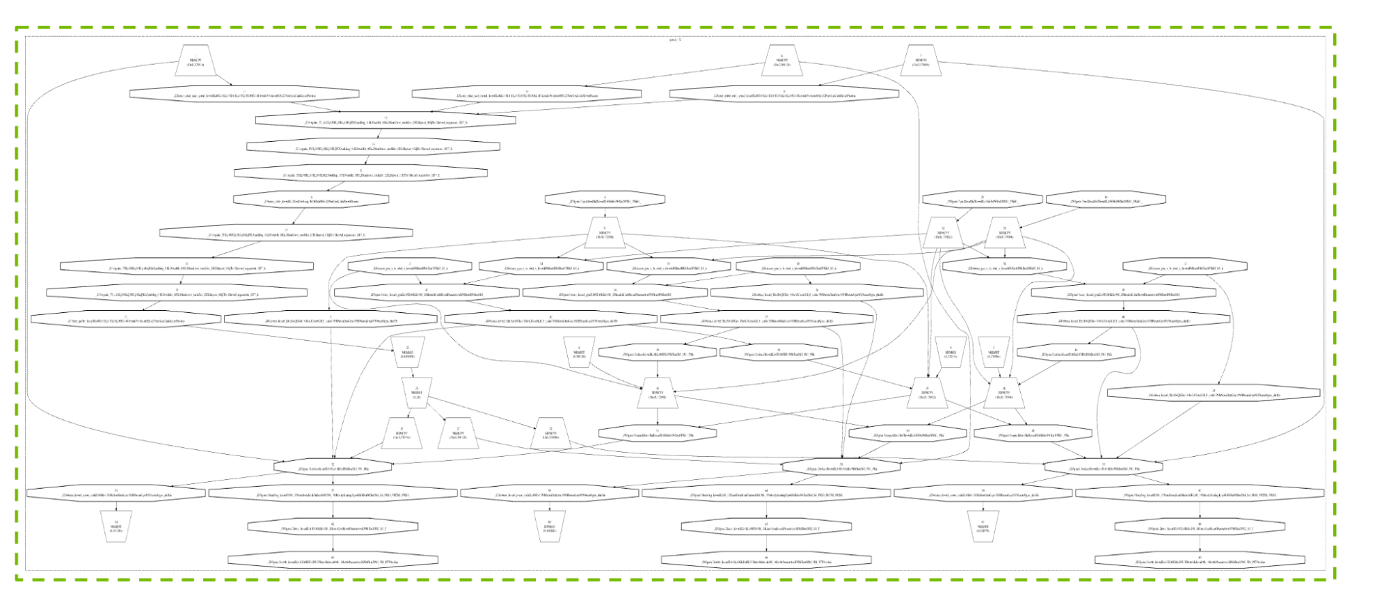 Figure 6. The real CUDA Graph for a 4-GPU case with three Particle-Particle GPUs and one Particle Mesh Ewald GPU, showing the overall complexity (not the details). Image obtained using cudaGraphDegugDotPrint
Development of the CUDA Graphs technology itself has been guided by GROMACS requirements, including support for graph update in conjunction with multi-threaded graph capture, and stream priority support within graphs. These enhancements will also ultimately benefit other applications.
Performance results
We used the Water Box set of benchmarks to demonstrate the benefits of CUDA Graphs in GROMACS. This set of benchmarks is available in the gromacs.org benchmark repository. It has the advantage of providing multiple atom counts, enabling assessment of how the performance behavior scales with system size.
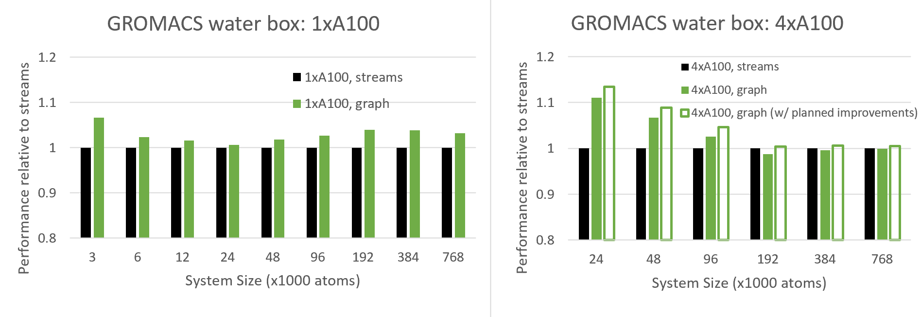 Figure 7. Comparison of the performance using CUDA Graphs against traditional streams, for water box systems configured with a range of atom counts, when using a single GPU (left) and four GPUs in parallel (right)
Figure 7 compares the performance of the new CUDA Graphs functionality with traditional streams, for varied system sizes, for both single-GPU and 4-GPUs runs.
Since CUDA graphs aim to reduce CPU API overheads, which are most notable for small cases, we expect to see increasing benefits at small system sizes, and we do indeed see this behavior for the multi-GPU case, and for 24K atoms and below for the single-GPU case.
Interestingly, for the single-GPU case above 24K atoms, the benefit actually increases with system size up to around 100K atoms where it plateaus. It can be seen that graphs offer a significant performance advantage over the full range of system sizes. This behavior needs more investigation, but we expect this is due to an added GPU-side benefit of CUDA Graphs where CUDA is more efficiently scheduling the thread blocks across multiple kernels when graphs are in use.
The benefits of graphs are more profound for the multi-GPU case, since (as described above) this configuration is more sensitive to CPU API overheads due to its complex scheduling. With the current version, we see benefits (for this case) up to around 100K atoms, where above this we see a slight degradation.
However, we also show projected results for a planned improvement which reduces an overhead associated with repeatedly re-building the graph. This improvement requires support in a future version of the CUDA driver, which is currently being improved in co-design with GROMACS. In general, we recommend that the user tries CUDA Graphs for their own case, and enables the feature where beneficial (see next section).
How to use CUDA Graphs in GROMACS
As mentioned above, this new CUDA Graphs feature is available for GPU-resident steps, which are typically invoked when all force and update calculations are offloaded to GPU through the following mdrun options:
-nb gpu -bonded gpu -pme gpu -update gpuWhen running with multiple tasks to enable multiple GPUs in parallel, GROMACS should be built using it’s internal thread-MPI library rather than an external MPI (-DGMX_MPI=OFF); GPU direct communication should be specified by setting the following environment variable:
export GMX_ENABLE_DIRECT_GPU_COMM=1A single PME GPU should be specified with -npme 1.
Then, CUDA Graphs can be triggered with the following:
export GMX_CUDA_GRAPH=1We recommend experimenting with any specific case, choosing to use graphs if it gives a performance advantage. Note that this remains an experimental feature which has had limited testing, so care should be taken to ensure the results are as expected (by comparing a scientific subset of results with and without use of graphs, for example). We welcome the reporting of any issues at the GROMACS GitLab site.
Summary
This post describes how we have integrated CUDA Graphs into GROMACS. This enables multiple GPU activities to be scheduled by the CPU in a single compute graph, which is more optimal than the traditional streams programming model. We demonstrated the benefits, including when running on multiple GPUs in parallel. The work is an important part of our ongoing efforts to modernize GROMACS with graph-based task scheduling, to aid the exploitation of increasingly complex hardware to solve increasingly complex scientific problems.
To get started, try activating CUDA Graphs for your own GROMACS case by following the instructions provided in this post.
Want to learn more? Join the GROMACS forum.
Source:: NVIDIA