A Comprehensive Overview of Regression Evaluation Metrics

GIXnews

1 year ago

As a data scientist, evaluating machine learning model performance is a crucial aspect of your work. To do so effectively, you have a wide range of statistical…

As a data scientist, evaluating machine learning model performance is a crucial aspect of your work. To do so effectively, you have a wide range of statistical metrics at your disposal, each with its own unique strengths and weaknesses. By developing a solid understanding of these metrics, you are not only better equipped to choose the best one for optimizing your model but also to explain your choice and its implications to business stakeholders.

In this post, I focus on metrics used to evaluate regression problems involved in predicting a numeric value—be it the price of a house or a forecast for next month’s company sales. As regression analysis can be considered the foundation of data science, it is essential to understand the nuances.

A quick primer on residuals

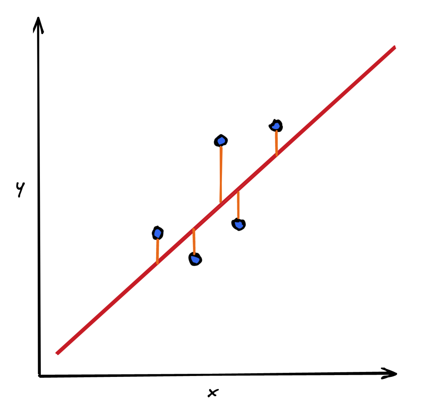
Residuals are the building blocks of the majority of the metrics. In simple terms, a residual is a difference between the actual value and the predicted value.

residual = actual - prediction

Figure 1 presents the relationship between a target variable (y) and a single feature (x). The blue dots represent observations. The red line is the fit of a machine learning model, in this case, a linear regression. The orange line represents the difference between the observed value and the prediction for that observation. As you can see, the residuals are calculated for each observation in the sample, be it the training or test set.

Line graph showing the residuals of a linear model Figure 1. Example of residuals in a linear model with one feature

Regression evaluation metrics

This section discusses some of the most popular regression evaluation metrics that can help you assess the effectiveness of your model.

Bias

The simplest error measure would be the sum of residuals, sometimes referred to as bias. As the residuals can be both positive (prediction is smaller than the actual value) and negative (prediction is larger than the actual value), bias generally tells you whether your predictions were higher or lower than the actuals.

However, as the residuals of opposing signs offset each other, you can obtain a model that generates predictions with a very low bias, while not being accurate at all.

Alternatively, you can calculate the average residual, or mean bias error (MBE).

R-squared

The next metric is likely the first one you encounter while learning about regression models, especially if that is during statistics or econometrics classes. R-squared (R²), also known as the coefficient of determination, represents the proportion of variance explained by a model. To be more precise, R² corresponds to the degree to which the variance in the dependent variable (the target) can be explained by the independent variables (features).

The following formula is used to calculate R²:

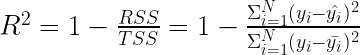
$R^2 = 1-frac{RSS}{TSS} = 1-frac{Sigma^N_{i=1} (y_i-hat{y_i})^2}{Sigma^N_{i=1} (y_i-bar{y_i})^2}$

RSS is the residual sum of squares, which is the sum of squared residuals. This value captures the prediction error of a model.
TSS is the total sum of squares. To calculate this value, assume a simple model in which the prediction for each observation is the mean of all the observed actuals. TSS is proportional to the variance of the dependent variable, as $frac{TSS}{N}$ is the actual variance of y where N is the number of observations. Think of TSS as the variance that a simple mean model cannot explain.

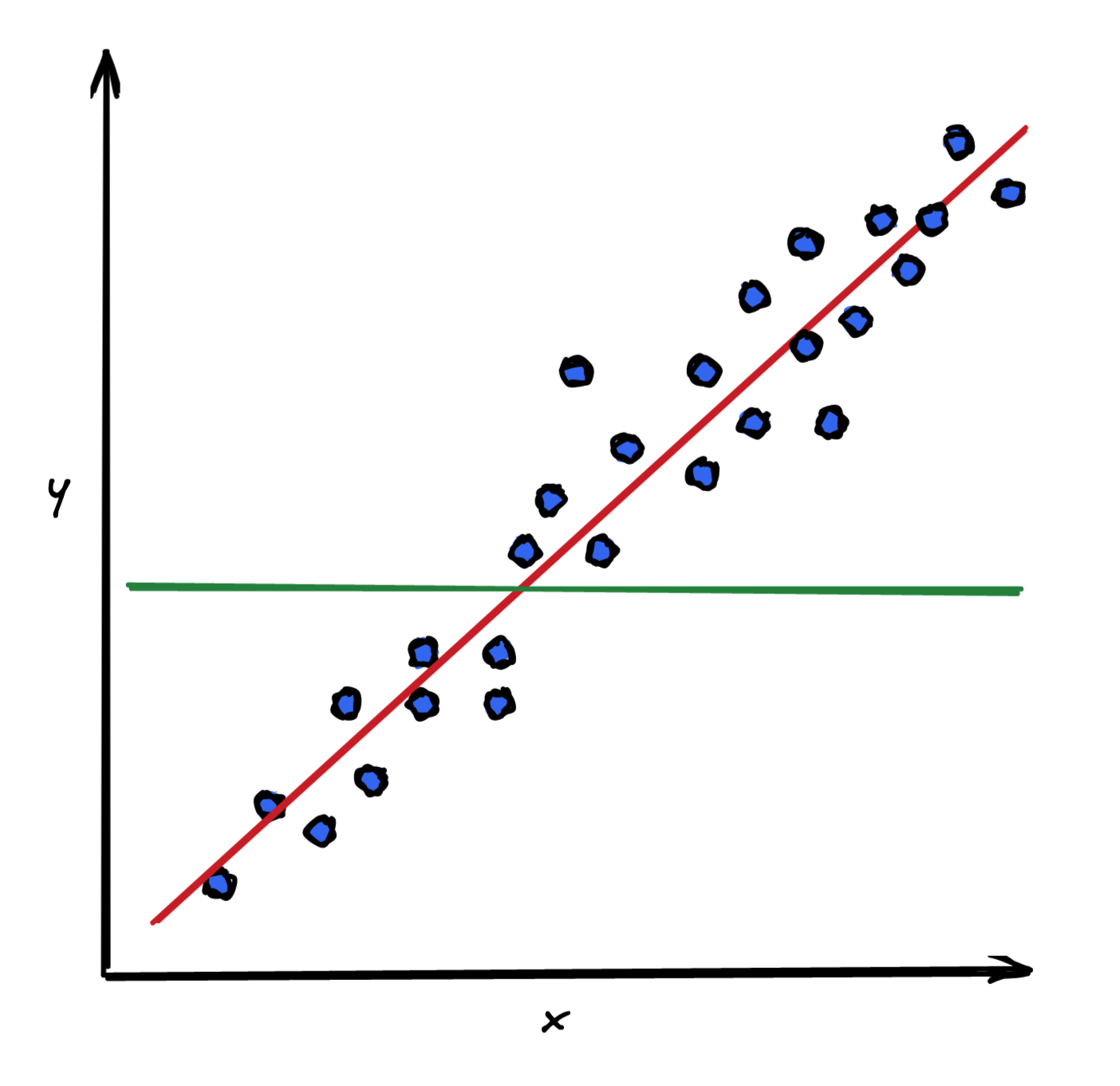
Effectively, you are comparing the fit of a model (represented by the red line in Figure 2) to that of a simple mean model (represented by the green line).

Line graph showing the comparison of a linear model’s fit to a mean benchmark Figure 2. Comparing the fit of a linear model to a simple mean benchmark

Knowing what the components of R² stand for, you can see that $frac{RSS}{TSS}$ represents the fraction of the total variance in the target that your model was not able to explain.

Here are some additional points to keep in mind when working with R².

R² is a relative metric; that is, it can be used to compare with other models trained on the same dataset. A higher value indicates a better fit.

R² can also be used to get a rough estimate of how the model performs in general. However, be careful when using R² for such evaluations:

First, different fields (social sciences, biology, finance, and more) consider different values of R² as good or bad.
Second, R² does not give any measure of bias, so you can have an overfitted (highly biased) model with a high value of R². As such, you should also look at other metrics to get a good understanding of a model’s performance.

A potential drawback of R² is that it assumes that every feature helps in explaining the variation in the target, when that might not always be the case. For this reason, if you continue adding features to a linear model estimated using ordinary least squares (OLS), the value of R² might increase or remain unchanged, but it never decreases.

Why? By design, OLS estimation minimizes the RSS. Suppose a model with an additional feature does not improve the value of R² of the first model. In that case, the OLS estimation technique sets that feature’s coefficients to zero (or some statistically insignificant value). In turn, this effectively brings you back to the initial model. In the worst-case scenario, you can get the score of your starting point.

A solution to the problem mentioned in the previous point is the adjusted R², which additionally penalizes adding features that are not useful for predicting the target. The value of the adjusted R² decreases if the increase in the R² caused by adding new features is not significant enough.

If a linear model is fitted using OLS, the range of R² is 0 to 1. That is because when using the OLS estimation (which minimizes the RSS), the general property is that RSS ≤ TSS. In the worst-case scenario, OLS estimation would result in obtaining the mean model. In that case, RSS would be equal to TSS and result in the minimum value of R² being 0. On the other hand, the best case would be RSS = 0 and R² = 1.

In the case of non-linear models, it is possible that R² is negative. As the model fitting procedure of such models is not based on iteratively minimizing the RSS, the fitted model could have an RSS greater than the TSS. In other words, the model’s predictions fit the data worse than the simple mean model. For more, information, see When is R squared negative?

Bonus: Using R², you can evaluate how much better your model fits the data as compared to the simple mean model. Think of a positive R² value in terms of improving the performance of a baseline model—something along the lines of a skill score. For example, R² of 40% indicates that your model has reduced the mean squared error by 40% compared to the baseline, which is the mean model.

Mean squared error

Mean squared error (MSE) is one of the most popular evaluation metrics. As shown in the following formula, MSE is closely related to the residual sum of squares. The difference is that you are now interested in the average error instead of the total error.

$MSE = frac{1}{N} Sigma^N_{i=1} (y_i-hat{y_i})^2$

Here are some points to take into account when working with MSE:

MSE uses the mean (instead of the sum) to keep the metric independent of the dataset size.
As the residuals are squared, MSE puts a significantly heavier penalty on large errors. Some of those might be outliers, so MSE is not robust to their presence.
As the metric is expressed using squares, sums, and constants ( $frac{1}{N}$ ), it is differentiable. This is useful for optimization algorithms.
While optimizing for MSE (setting its derivative to 0), the model aims for the total sum of predictions to be equal to the total sum of actuals. That is, it leads to predictions that are correct on average. Therefore, they are unbiased.
MSE is not measured in the original units, which can make it harder to interpret.
MSE is an example of a scale-dependent metric, that is, the error is expressed in the units of the underlying data (even though it actually needs a square root to be expressed on the same scale). Therefore, such metrics cannot be used to compare the performance between different datasets.

Root mean squared error

Root mean squared error (RMSE) is closely related to MSE, as it is simply the square root of the latter. Take the square to bring the metric back to the scale of the target variable, so it is easier to interpret and understand. However, take caution: one fact that is often overlooked is that although RMSE is on the same scale as the target, an RMSE of 10 does not actually mean you are off by 10 units on average.

$RMSE = sqrt{frac{1}{N} Sigma^N_{i=1} (y_i-hat{y_i})^2}$

Other than the scale, RMSE has the same properties as MSE. As a matter of fact, optimizing for RMSE while training a model will result in the same model as that obtained while optimizing for MSE.

Mean absolute error

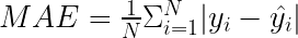
The formula to calculate mean absolute error (MAE) is similar to the MSE formula. Replace the square with the absolute value.

$MAE = frac{1}{N} Sigma^N_{i=1} |y_i-hat{y_i}|$

Characteristics of MAE include the following:

Due to the lack of squaring, the metric is expressed at the same scale as the target variable, making it easier to interpret.
All errors are treated equally, so the metric is robust to outliers.
Absolute value disregards the direction of the errors, so underforecasting = overforecasting.
Similar to MSE and RMSE, MAE is also scale-dependent, so you cannot compare it between different datasets.
When you optimize for MAE, the prediction must be as many times higher than the actual value as it should be lower. That means that you are effectively looking for the median; that is, a value that splits a dataset into two equal parts.
As the formula contains absolute values, MAE is not easily differentiable.

Mean absolute percentage error

Mean absolute percentage error (MAPE) is one of the most popular metrics on the business side. That is because it is expressed as a percentage, which makes it much easier to understand and interpret.

$MAPE = frac{1}{N} Sigma^N_{i=1} |frac{y_i-hat{y_i}}{y_i}|$

To make the metric even easier to read, multiply it by 100% to express the number as a percentage.

Points to consider:

MAPE is expressed as a percentage, which makes it a scale-independent metric. It can be used to compare predictions on different scales.
MAPE can exceed 100%.
MAPE is undefined when the actuals are zero (division by zero). Additionally, it can take extreme values when the actuals are very close to zero.
MAPE is asymmetric and puts a heavier penalty on negative errors (when predictions are higher than actuals) than on positive ones. This is caused by the fact that the percentage error cannot exceed 100% for forecasts that are too low. Meanwhile, there is no upper limit for forecasts that are too high. As a result, optimizing for MAPE will favor models that underforecast rather than overforecast.
Hyndman (2021) elaborates on the often-forgotten assumption of MAPE; that is, the unit of measurement of the variable has a meaningful zero value. As such, forecasting demand and using MAPE do not raise any red flags. However, you will encounter that problem when forecasting temperature expressed on the Celsius scale (and not only that one). That is because the temperature has an arbitrary zero point and it does not make sense to talk about percentages in their context.
MAPE is not differentiable everywhere, which can result in problems while using it as the optimization criterion.
As MAPE is a relative metric, the same error can result in a different loss depending on the actual value. For example, for a predicted value of 60 and an actual of 100, the MAPE would be 40%. For a predicted value of 60 and an actual of 20, the nominal error is still 40, but on the relative scale, it is 300%.
Unfortunately, MAPE does not provide a good way to differentiate the important from the irrelevant. Assume you are working on demand forecasting and over a horizon of a few months, you get a MAPE of 10% for two different products. Then, it turns out that the first product sells an average of 1 million units per month, while the other only 100. Both have the same 10% MAPE. When aggregating over all products, those two would contribute equally, which can be far from desirable. In such cases, it makes sense to consider weighted MAPE (wMAPE).

Symmetric mean absolute percentage error

While discussing MAPE, I mentioned that one of its potential drawbacks is its asymmetry (not limiting the predictions that are higher than the actuals). Symmetric mean absolute percentage error (sMAPE) is a related metric that attempts to fix that issue.

$sMAPE = frac{1}{N} Sigma^N_{i=1} frac{|y_i-hat{y_i}|}{(y_i+hat{y_i})/2}$

Points to consider when using sMAPE:

It is expressed as a bounded percentage, that is, it has lower (0%) and upper (200%) bounds.
The metric is still unstable when both the true value and the forecast are very close to zero. When it happens, you will deal with division by a number very close to zero.
The range of 0% to 200% is not intuitive to interpret. Dividing by two in the denominator is often omitted.
Whenever the actual value or the forecast has a value is 0, sMAPE will automatically hit the upper boundary value.
sMAPE includes the same assumptions as MAPE regarding a meaningful zero value.
While fixing the asymmetry of boundlessness, sMAPE introduces another kind of delicate asymmetry caused by the denominator of the formula. Imagine two cases. In the first one, you have A = 100 and F = 120. The sMAPE is 18.2%. Now a similar case, in which you have A = 100 and F = 80, the sMAPE is 22.2%. As such, sMAPE tends to penalize underforecasting more severely than overforecasting.
sMAPE might be one of the most controversial error metrics, especially in time series forecasting. That is because there are at least a few versions of this metric in the literature, each one with slight differences that impact its properties. Finally, the name of the metric suggests that there is no asymmetry, but that is not the case.

Other regression evaluation metrics to consider

I have not described all the possible regression evaluation metrics, as there are dozens (if not hundreds). Here are a few more metrics to consider while evaluating models:

Mean squared log error (MSLE) is a cousin of MSE, with the difference that you take the log of the actuals and predictions before calculating the squared error. Taking the logs of the two elements in subtraction results in measuring the ratio or relative difference between the actual value and the prediction, while neglecting the scale of the data. That is why MSLE reduces the impact of outliers on the final score. MSLE also puts a heavier penalty on underforecasting.
Root mean squared log error (RMSLE) is a metric that takes the square root of MSLE. It has the same properties as MSLE.
Akaike information criterion (AIC) and Bayesian information criterion (BIC) are examples of information criteria. They are used to find a balance between a good fit and the complexity of a model. If you start with a simple model with a few parameters and add more, your model will probably fit the training data better. However, it will also grow in complexity and risk overfitting. On the other hand, if you start with many parameters and systematically remove some of them, the model becomes simpler. At the same time, you reduce the risk of overfitting at the potential cost of losing on performance (goodness of fit). The difference between AIC and BIC is the weight of the penalty for complexity. Keep in mind that it is not valid to compare the information criteria on different datasets or even subsamples of the same dataset but with a different number of observations.

When to use each evaluation metric

As with the majority of data science problems, there is no single best metric for evaluating the performance of a regression model. The metric chosen for a use case will depend on the data used to train the model, the business case you are trying to help, and so on. For this reason, you might often use a single metric for the training of a model (the metric optimized for), but when reporting to stakeholders, data scientists often present a selection of metrics.

While choosing the metrics, consider a few of the following questions:

Do you expect frequent outliers in the dataset? If so, how do you want to account for them?
Is there a business preference for overforecasting or underforecasting?
Do you want a scale-dependent or scale-independent metric?

I believe it is useful to explore the metrics on some toy cases to fully understand their nuances. While most of the metrics are available in the metrics module of scikit-learn, for this particular task, the good old spreadsheets might be a more suitable tool.

The following example contains five observations. Table 1 shows the actual values, predictions, and some metrics used to calculate most of the considered metrics.

yy_hatresidualsquared errorabs errorabs perc errorsAPE100120-204002020.00%18.18%10080204002020.00%22.22%80100-204002025.00%22.22%200240-401,6004020.00%18.18%4053512253587.50%155.56%Table 1. Example of calculating the performance metrics on five observations

MSE805RMSE28.37MAE27MAPE34.50%sMAPE47.27%Table 2. Performance metrics calculated using the values in Table 1

The first three rows contain scenarios in which the absolute difference between the actual value and the prediction is 20. The first two rows show an overforecast and underforecast of 20, with the same actual. The third row shows an overforecast of 20, but with a smaller actual. In those rows, it is easy to observe the particularities of MAPE and sMAPE.

The fifth row in Table 1 contained a prediction 8x smaller than the actual value. For the sake of experimentation, replace that prediction with one that is 8x higher than the actual. Table 3 contains the revised observations.

yy_hatresidualsquared errorabs errorabs perc errorsAPE100120-204002020.00%18.18%10080204002020.00%22.22%80100-204002025.00%22.22%200240-401,6004020.00%18.18%40320-28078,400280700.00%155.56%Table 3. Performance metrics after modifying a single observation to be more extreme

MSE16240RMSE127.44MAE76MAPE157.00%sMAPE47.27%Table 4. Performance metrics calculated using the modified values in Table 3

Basically, all metrics exploded in size, which is intuitively consistent. That is not the case for sMAPE, which stayed the same between both cases.

I highly encourage you to play around with such toy examples to more fully understand how different kinds of scenarios impact the evaluation metrics. This experimentation should make you more comfortable making a decision on which metric to optimize for and the consequences of such a choice. These exercises might also help you explain your choices to stakeholders.

Summary

In this post, I covered some of the most popular regression evaluation metrics. As explained, each one comes with its own set of advantages and disadvantages. And it is up to the data scientist to understand those and make a choice about which one (or more) is suitable for a particular use case. The metrics mentioned can also be applied to pure regression tasks—such as predicting salary based on a selection of features connected to experience—but also to the domain of time series forecasting.

If you are looking to build robust linear regression models that can handle outliers effectively, see my previous post, Dealing with Outliers Using Three Robust Linear Regression Models.

References

Jadon, A., Patil, A., & Jadon, S. (2022). A Comprehensive Survey of Regression Based Loss Functions for Time Series Forecasting. arXiv preprint arXiv:2211.02989.

Hyndman, R. J. (2006). Another look at forecast-accuracy metrics for intermittent demand. Foresight: The International Journal of Applied Forecasting, 4(4), 43-46.

Hyndman, R. J., & Koehler, A. B. (2006). Another look at measures of forecast accuracy. International journal of forecasting, 22(4), 679-688.

Hyndman, R.J., & Athanasopoulos, G. (2021) Forecasting: principles and practice, 3rd edition, OTexts: Melbourne, Australia. OTexts.com/fpp3.

Source:: NVIDIA