
Linear regression is a powerful statistical tool used to model the relationship between a dependent variable and one or more independent variables (features)….
Linear regression is a powerful statistical tool used to model the relationship between a dependent variable and one or more independent variables (features). An important, and often forgotten, concept in regression analysis is that of interaction terms. In short, interaction terms enable you to examine whether the relationship between the target and the independent variable changes depending on the value of another independent variable.
Interaction terms are a crucial component of regression analysis, and understanding how they work can help practitioners better train models and interpret their data. Despite their importance, however, interaction terms can be difficult to understand.
This post provides an intuitive explanation of interaction terms in the context of linear regression.
What are interaction terms in regression models?
First, here’s the simpler case; that is, a linear model without interaction terms. Such a model assumes that the effect of each feature or predictor on the dependent variable (target) is independent of other predictors in the model.
The following equation describes such a model specification with two features:

To make the explanation easier to understand, here’s an example. Imagine that you are interested in modeling the price of real estate properties (y) using two features: their size (X1) and a Boolean flag indicating whether the apartment is located in the city center (X2). 


After gathering data and estimating a linear regression model, you obtain the following coefficients:

Knowing the estimated coefficients and that X2 is a Boolean feature, you can write out the two possible scenarios depending on the value of X2.
City center
Outside of the city center
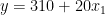
How to interpret those? While this might not make a lot of sense in the context of real estate, you can say that a 0-square-meter apartment in the city center costs 310 (the value of the intercept). Each square meter of additional space increases the price by 20. In the other case, the only difference is that the intercept is smaller by 10 units. Figure 1 shows the two best-fit lines.
 Figure 1. Regression lines for properties in the city center and outside of it
As you can see, the lines are parallel and they have the same slope — the coefficient by X1, which is the same in both scenarios.
Interaction terms represent joint effects
At this point, you might argue that an additional square meter in an apartment in the city center costs more than an additional square meter in an apartment on the outskirts. In other words, there might be a joint effect of these two features on the price of real estate.
So, you believe that not only the intercept should be different between the two scenarios but also the slope of the lines. How to do that? That is exactly when the interaction terms come into play. They make the models’ specifications more flexible and enable you to account for such patterns.
An interaction term is effectively a multiplication of the two features that you believe have a joint effect on the target. The following equation presents the model’s new specification:

Again, assume that you have estimated your model and you know the coefficients. For simplicity, I’ve kept the same values as in the previous example. Bear in mind that in a real-life scenario, they would likely differ.

City center
Outside of the city center
After you write out the two scenarios for X2 (city center or outside of the city center), you can immediately see that the slope (coefficient by X1) of the two lines is different. As hypothesized, an additional square meter of space in the city center is now more expensive than in the suburbs.
Interpreting the coefficients with interaction terms
Adding interaction terms to a model changes the interpretation of all the coefficients. Without an interaction term, you interpret the coefficients as the unique effect of a predictor on the dependent variable.
So in this case, you could say that
To better understand what each coefficient represents, here’s one more look at the raw specification of a linear model with interaction terms. Just as a reminder, X2 is a Boolean feature indicating whether a particular apartment is in the city center.
Now, you can interpret each of the coefficients in the following way:
: Difference in slopes between apartments in the city center and outside of it.
For example, assume that you are testing a hypothesis that there is an equal impact of the size of an apartment on its price, regardless of whether the apartment is in the city center. Then, you would estimate the linear regression with the interaction term and check whether
Some additional notes on the interaction terms:
- I’ve presented two-way interaction terms; however, higher-order interactions (for example, of three features) are also possible.
- In this example, I showed an interaction of a numerical feature (size of the apartment) with a Boolean one (is the apartment in the city center?). However, you can create interaction terms for two numerical features as well. For example, you might create an interaction term of the size of the apartment with the number of rooms. For more information, see the Related resources section.
- It might be the case that the interaction term is statistically significant, but the main effects are not. Then, you should follow the hierarchical principle stating that if you include an interaction term in the model, you should also include the main effects, even if their impacts are not statistically significant.
Hands-on example in Python
After all the theoretical introduction, here’s how to add interaction terms to a linear regression model in Python. As always, start by importing the required libraries.
import numpy as np
import pandas as pd

import statsmodels.api as sm
import statsmodels.formula.api as smf

# plotting
import seaborn as sns
import matplotlib.pyplot as plt

# settings
plt.style.use("seaborn-v0_8")
sns.set_palette("colorblind")
plt.rcParams["figure.figsize"] = (16, 8)
%config InlineBackend.figure_format = 'retina'
In this example, you estimate linear models using the statsmodels library. For the dataset, use the mtcars dataset. I am quite sure that if you have ever worked with R, you will be already familiar with this dataset.
First, load the dataset:
mtcars = sm.datasets.get_rdataset("mtcars", "datasets", cache=True)
print(mtcars.__doc__)
Executing the code example prints a comprehensive description of the dataset. In this post, I only show the relevant parts — an overall description and the definition of the columns:
  ====== ===============
  mtcars R Documentation
  ====== ===============
The data was extracted from the 1974 US magazine MotorTrend, and is composed of fuel consumption and 10 aspects of automobile design and performance for 32 automobiles (1973–74 models).
Here’s a DataFrame with 32 observations on 11 (numeric) variables:
  ===== ==== ========================================
  [, 1] mpg  Miles/(US) gallon
  [, 2] cyl  Number of cylinders
  [, 3] disp Displacement (cu.in.)
  [, 4] hp   Gross horsepower
  [, 5] drat Rear axle ratio
  [, 6] wt   Weight (1000 lbs)
  [, 7] qsec 1/4 mile time
  [, 8] vs   Engine (0 = V-shaped, 1 = straight)
  [, 9] am   Transmission (0 = automatic, 1 = manual)
  [,10] gear Number of forward gears
  [,11] carb Number of carburetors
  ===== ==== ========================================
Then, extract the actual dataset from the loaded object:
df = mtcars.data
df.head()
mpgcyldisphpdratwtqsecvsamgearcarbMazda RX421.061601103.902.62016.460144Mazda RX4 Wag21.061601103.902.87517.020144Datsun 71022.84108933.852.32018.611141Hornet 4 Drive21.462581103.083.21519.441031Hornet Sportabout18.783601753.153.44017.020032Table 1. A preview of the mtcars dataset
For this example, assume that you want to investigate the relationship between the miles per gallon (mpg) and two features: weight (wt, continuous) and type of transmission (am, Boolean).
First, plot the data to get some initial insights:
sns.lmplot(x="wt", y="mpg", hue="am", data=df, fit_reg=False)
plt.ylabel("Miles per Gallon")
plt.xlabel("Vehicle Weight");
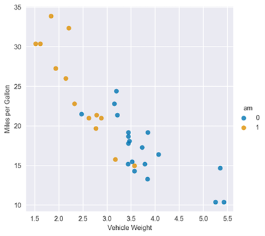 Figure 2. Scatterplot of miles per gallon vs. vehicle weight, color per transmission type
Just by eyeballing Figure 2, you can see that the regression lines for the two categories of the am variable will be quite different. For comparison’s sake, start off with a model without interaction terms.
model_1 = smf.ols(formula="mpg ~ wt + am", data=df).fit()
model_1.summary()
The following tables show the results of fitting a linear regression without the interaction term.
OLS Regression Results
==============================================================================
Dep. Variable:                	  mpg   	R-squared:             	0.753
Model:                        	  OLS      Adj. R-squared:             	0.736
Method:                 Least Squares         F-statistic:             	44.17
Date:                Sat, 22 Apr 2023  Prob (F-statistic):           1.58e-09
Time:                        23:15:11      Log-Likelihood:            -80.015
No. Observations:              	   32   	      AIC:      	166.0
Df Residuals:                  	   29  	              BIC:          	170.4
Df Model:           	            2
Covariance Type:            nonrobust
==============================================================================
               coef     std err         t      P>|t|       [0.025       0.975]
------------------------------------------------------------------------------
Intercept   37.3216  	  3.055    12.218      0.000       31.074  	43.569
wt          -5.3528  	  0.788    -6.791      0.000       -6.965  	-3.741
am          -0.0236  	  1.546    -0.015      0.988       -3.185        3.138
==============================================================================
Omnibus:                    	3.009   Durbin-Watson:                  1.252
Prob(Omnibus):                  0.222   Jarque-Bera (JB):            	2.413
Skew:                       	0.670   Prob(JB):                    	0.299
Kurtosis:                   	2.881   Cond. No.                      21.7
==============================================================================
From the summary tables, you can see that the coefficient by the am feature is not statistically significant. Using the interpretation of the coefficients you’ve already learned, you can plot the best-fit lines for both classes of the am feature.
X = np.linspace(1, 6, num=20)
sns.lmplot(x="wt", y="mpg", hue="am", data=df, fit_reg=False)
plt.title("Best fit lines for from the model without interactions")
plt.ylabel("Miles per Gallon")
plt.xlabel("Vehicle Weight")
plt.plot(X, 37.3216 - 5.3528 * X, "blue")
plt.plot(X, (37.3216 - 0.0236) - 5.3528 * X, "orange");
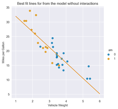 Figure 3. Best-fit lines for both types of transmission
Figure 3 shows that the lines are almost overlapping, as the coefficient by the am feature is basically zero.
Follow up with a second model, this time with an interaction term between the two features. Here’s how to add an interaction term as an additional input in the statsmodels formula.
model_2 = smf.ols(formula="mpg ~ wt + am + wt:am", data=df).fit()
model_2.summary()
The following summary tables show the results of fitting a linear regression with the interaction term.
OLS Regression Results
==============================================================================
Dep. Variable:                	 mpg      R-squared:                  0.833
Model:                        	 OLS      Adj. R-squared:             0.815
Method:                Least Squares      F-statistic:               46.57
Date:               Mon, 24 Apr 2023      Prob (F-statistic):         5.21e-11
Time:                       21:45:40      Log-Likelihood:           -73.738
No. Observations:              	  32      AIC:                      155.5
Df Residuals:                  	  28      BIC:                      161.3
Df Model:                          3
Covariance Type:           nonrobust
===============================================================================
                coef     std err         t      P>|t|       [0.025       0.975]
------------------------------------------------------------------------------
Intercept    31.4161  	   3.020    10.402  	0.000  	    25.230  	 37.602
wt           -3.7859  	   0.786    -4.819  	0.000  	    -5.395  	 -2.177
am           14.8784  	   4.264     3.489  	0.002        6.144  	 23.613
wt:am        -5.2984  	   1.445    -3.667  	0.001  	    -8.258  	 -2.339
==============================================================================
Omnibus:                    	3.839   Durbin-Watson:               	1.793
Prob(Omnibus):              	0.147   Jarque-Bera (JB):            	3.088
Skew:                       	0.761   Prob(JB):                    	0.213
Kurtosis:                   	2.963   Cond. No.                      40.1
==============================================================================
Here are two conclusions that you can quickly draw from the summary tables with the interaction term:
- All the coefficients, including the interaction term, are statistically significant.
- By inspecting the R2 (and its adjusted variant, as you have a different number of features in the models), you can state that the model with the interaction term results in a better fit.
Similarly to the previous case, plot the best-fit lines:
X = np.linspace(1, 6, num=20)
sns.lmplot(x="wt", y="mpg", hue="am", data=df, fit_reg=False)
plt.title("Best fit lines for from the model with interactions")
plt.ylabel("Miles per Gallon")
plt.xlabel("Vehicle Weight")
plt.plot(X, 31.4161 - 3.7859 * X, "blue")
plt.plot(X, (31.4161 + 14.8784) + (-3.7859 - 5.2984) * X, "orange");
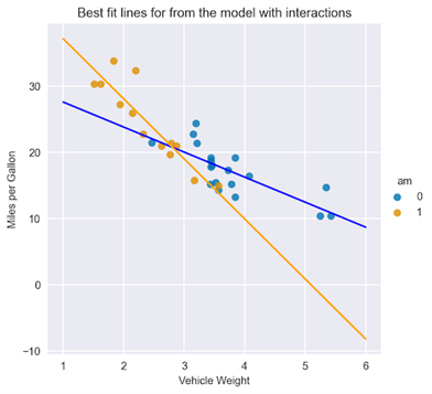 Figure 4. Best fit lines for both types of transmission, including interaction terms
In Figure 4, you can immediately see the difference in the fitted lines, both in terms of the intercept and the slope, for cars with automatic and manual transmissions.
Here’s a bonus: You can also add interaction terms using scikit-learn’s PolynomialFeatures. The transformer offers not only the possibility to add interaction terms of arbitrary order, but it also creates polynomial features (for example, squared values of the available features). For more information, see sklearn.preprocessing.PolynomialFeatures.
Wrapping up
When working with interaction terms in linear regression, there are a few things to remember:
- Interaction terms enable you to examine whether the relationship between the target and a feature changes depending on the value of another feature.
- Add interaction terms as a multiplication of the original features. By adding these new variables to the regression model, you can measure the effects of the interaction between them and the target. It is crucial to interpret the coefficients of the interaction terms carefully to understand the direction and the strength of the relationship.
- By using interaction terms, you can make the specification of a linear model more flexible (different slopes for different lines), which can result in a better fit to the data and better predictive performance.
You can find the code used in this post in my /erykml GitHub repo. As always, any constructive feedback is more than welcome. You can reach out to me on Twitter or in the comments below.
Related resources
- Interpreting Interactions OLS
- Interactions between continuous variables
- Chapter 13: Plotting Regression Interactions
- Exploring Linear Regression Coefficients and Interactions
Source:: NVIDIA