
A retailer’s supply chain includes the sourcing of raw materials or finished goods from suppliers; storing them in warehouses or distribution centers; and…
A retailer’s supply chain includes the sourcing of raw materials or finished goods from suppliers; storing them in warehouses or distribution centers; and transporting them to stores or customers; managing sales. They also collect, store, and analyze data to optimize supply chain performance.
Retailers have teams responsible for managing each stage of the supply chain, including supplier management, logistics, inventory management, sales, and data analytics. All these teams and processes work together to ensure that the right products are available to customers at the right time and at the right price.
It is important to make informed decisions about retail sales and operations by collecting, analyzing, and interpreting data from various sources, such as point-of-sale (POS) systems, customer databases, and market research surveys.
Big data processing is a key component of retail analytics, as it enables retailers to handle and analyze large volumes of data from various sources with low latency. Retailers can gain valuable insights into customer behavior, market trends, and operational efficiency.
This post provides an overview of retail applications that can benefit from GPU-accelerated Apache Spark workloads. We provide detailed step-by-step instructions with a sample retail use case on how to get started with using GPU acceleration on Spark workloads on Dataproc. The example shows you how to speed up data processing pipelines for retailers. We highlight new RAPIDS Accelerator user tools for Dataproc that help set you up for application tuning and also provide insights into GPU run details.
To follow along with this post, access the notebook on the NVIDIA/spark-rapids-examples GitHub repository.
Types of data analysis for retail applications
Depending on your business questions and goals, several types of complex analysis can be performed on retail data:
- Inventory forecasting: Analyzing the sales trend, demand, and quantity in stock to predict future inventory needs.
- Demand forecasting: Predicting future customer demand for products to optimize inventory levels, pricing, and promotions to meet that demand.
- Price optimization: Analyzing the competitor’s price, cost of goods, and transportation cost to determine the optimal price for each product.
- Sales performance analysis: Analyzing the sales status and purchase history of individual customers to identify patterns and target marketing efforts.
- Supply chain analysis: Analyzing the supplier ID, shipping cost, and warehouse cost to identify opportunities for cost savings and efficiency improvements.
- Customer segmentation: Analyzing the customer demographics, purchase history, and contact information to segment customers and target marketing efforts.
- Product analysis: Analyzing the sales of different products and identifying top-selling products and potential new products to introduce.
- Location analysis: Analyzing the location of the sales and identifying potential new locations to expand to.
- Retail markdown optimization: Analyzing large amounts of data to replace the manual process of lowering product prices.
For instance, you can optimize in-store or online inventory levels by processing recent product sales data from different sources.
Retail data sources
Retail data can derive from a variety of sources:
- Sales data: Data on the products that are being sold, such as the product name, price, quantity sold, and date of sale. This data can come from POS systems, online sales platforms, or other systems where the sales transactions are recorded.
- Stock data: Data on the products that are currently in stock, such as the product name, quantity in stock, location of the stock, and the date it was received. This data can come from inventory management systems, warehouse management systems, or other systems where the stock is recorded.
- Supplier data: Data on the products that are being ordered from suppliers, such as the product name, quantity ordered, price, and the date the order was placed. This data can come from purchase order systems, supply chain management systems, or other systems where supplier orders are recorded.
- Customer data: Data on customers such as demographics, purchase history, and contact information. This data can come from customer relationship management (CRM) systems, e-commerce platforms, or other systems where customer information is recorded.
- Market data: Data on the market conditions, competitor’s prices, sales trends, and demand forecasts. This data can come from external sources such as market research firms, government agencies, or other data providers.
- Logistic data: Data on logistics such as shipping, transportation, and warehouse management. This data can come from logistics management systems, shipping carriers, or other systems where logistic information is recorded.
Data from these sources may be in different formats (CSV, JSON, Parquet, and so on).
In this post, you use a synthetic data generator code to mock up the data sources and formats explained earlier. The following Python code example can generate huge volumes of synthetic sales data, stock data, supplier data, customer data, market data, and logistic data in different formats. There are some data quality issues that can be used as an example for simulation purposes.
# generate sales data
# Define the generate_data function which takes an integer i as input and generates sales data using random numbers. The generated data includes sales ID, product name, price, quantity sold, date of sale, and customer ID. The function returns a tuple of the generated data. The multiprocessing library is used to generate the data in parallel

def generate_data(i):
    sales_id = "s_{}".format(i)
    product_name = "Product_{}".format(i)
    price = random.uniform(1,100)
    quantity_sold = random.randint(1,100)
    date_of_sale = "2022-{}-{}".format(random.randint(1,12), random.randint(1,28))
    customer_id = "c_{}".format(random.randint(1,1000000))
    return (sales_id, product_name, price, quantity_sold, date_of_sale, customer_id)

with mp.Pool(mp.cpu_count()) as p:
    sales_data = p.map(generate_data, range(100000000))
    sales_data = list(sales_data)

print("write to gcs started")
sales_df = pd.DataFrame(sales_data, columns=["sales_id", "product_name", "price", "quantity_sold", "date_of_sale", "customer_id"])
sales_df.to_csv(dataRoot+"sales/data.csv", index=False, header=True)
print("Write to gcs completed")
Access the full notebook on the spark-rapids-examples GitHub repository.
Data cleaning, transformation, and integration
The raw data may have to be cleaned, transformed, and integrated before it can be used for analysis. This is where Apache Spark SQL and DataFrame APIs come in, as they provide a powerful set of tools for working with structured data. They can handle large amounts of data from different sources to process and extract useful insights and information.
First, extract the data, which can be in different formats, such as CSV, JSON, or Parquet. Then, load data into Spark using the DataFrame API. Spark SQL is used to perform data cleaning and preprocessing tasks:
- Remove missing values.
- Handle outliers.
- Transform the data into a suitable format for analysis.
After the data is cleaned and preprocessed, use Spark SQL and DataFrame API to perform various types of analysis for inventory optimization.
For example, you can analyze sales data with SQL queries to identify top-selling and underperforming products. To perform advanced analysis, such as time series analysis, use the DataFrame API to forecast future demand and optimization algorithms or analyze purchase patterns in datasets.
Finally, apply analysis results to make decisions, such as how much stock to hold in inventory, how much to order from suppliers, and when to do so. Use Spark’s Dataframe API or integrate with other systems to update inventory levels automatically.
Also, using Spark SQL and DataFrame API to process large amounts of data from different sources such as sales, stock, and supplier data enables a more efficient and accurate inventory management system.
You can accelerate the process and save compute costs by running the data pipeline on a GPU-powered Google Dataproc cluster. The rest of this post is a step-by-step guide on the process of creating GPU-powered clusters and running the accelerated data processing pipeline using RAPIDS Accelerator.
Create a RAPIDS Accelerator GPU-enabled Dataproc cluster
Retailers’ various data sources push their raw data to Google Cloud Storage, which serves as a source for processing it on the GPU-enabled Dataproc cluster. In the Dataproc cluster, you can enable the Jupyter lab component gateway to run a notebook that performs data cleaning, merging, and analysis on top of the merged data.
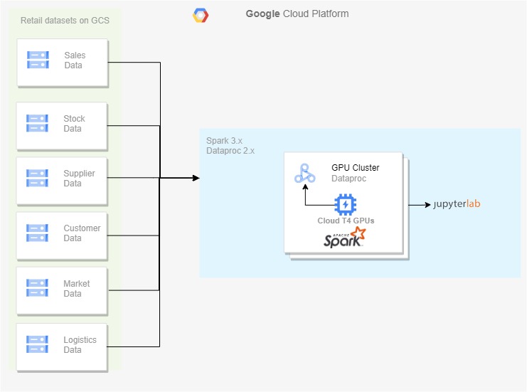 Figure 1. Retail data can be pulled from multiple sources
In Figure 1, I kept the generated retail source datasets on cloud storage and used the Dataproc 2.x cluster to process the data. GPU enablement with RAPIDS Accelerator can be done based on that process.
To create a GPU-enabled Dataproc cluster, run shell commands using Cloud Shell. To do this, first enable the Compute and Dataproc APIs to gain access to Dataproc. Also, enable the Storage API as you need a Google Cloud Storage bucket to store your data. This process may take a few minutes to complete.
gcloud services enable compute.googleapis.com
gcloud services enable dataproc.googleapis.com
gcloud services enable storage-api.googleapis.com
The following example configurations help you run GPU-enabled workloads on GCP. Adjust the sizes and number of GPU based on your needs.
To launch a GPU-enabled cluster with RAPIDS Accelerator, run the following command in the CLI:
gcloud dataproc clusters create sparkrapidsnew
--region us-central1
--subnet default
--zone us-central1-c
--master-machine-type n1-standard-8
--master-boot-disk-size 500
--num-workers 4
--worker-machine-type n1-standard-8
--worker-boot-disk-size 1000
--worker-accelerator type=nvidia-tesla-t4,count=2
--image-version 2.0-debian10
--properties spark:spark.eventLog.enabled=true,spark:spark.ui.enabled=true
--optional-components HIVE_WEBHCAT,JUPYTER,ZEPPELIN,ZOOKEEPER
--project PROJECT_NAME
--initialization-actions=gs://goog-dataproc-initialization-actions-us-central1/spark-rapids/spark-rapids.sh --metadata gpu-driver-provider="NVIDIA"
--enable-component-gateway
Figure 2 shows creating a GPU cluster with one T4 GPU each on the worker nodes. The script in the initialization actions installs the latest version of RAPIDS Accelerator libraries in the cluster.
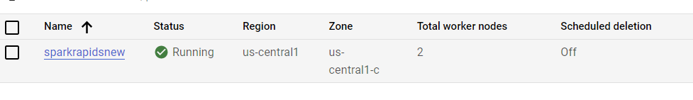 Figure 2. The resulting GPU-enabled cluster
You can also build a custom dataproc image to accelerate cluster init time. For more information, see the Getting started with RAPIDS Accelerator on GCP Dataproc quick start page.
Run PySpark on Jupyter Lab
To use notebooks with a Dataproc cluster, select the cluster under the Dataproc cluster and choose Web Interfaces, Jupyter Lab.
Data cleansing
Run the following command to complete these tasks:
# remove missing values
sales_df = sales_df.dropDuplicates()
# remove duplicate data
sales_df = salesdf.dropna()
# convert date columns to date type
sales_df = sales_df.withColumn("date_of_sale", to_date(col("date_of_sale")))
# standardize case of string columns
sales_df = sales_df.withColumn("product_name", upper(col("product_name")))
# remove leading and trailing whitespaces
sales_df = sales_df.withColumn("product_name", trim(col("product_name")))
# check for invalid values
sales_df = sales_df.filter(col("product_name").isNotNull())
After you’ve cleaned the data, join all the data on a common column (product_name or customer_name) and write the cleaned and transformed data to the Parquet file format.
This is an example of how PySpark can be used to perform data cleaning and preprocessing tasks on large datasets. However, keep in mind that the specific cleaning and preprocessing steps vary depending on the nature of the data and the requirements of the analysis.
Retail data analysis
You can perform various retail data analytics using PySpark. In the demo notebook, PySpark is reading cleaned data in Apache Parquet format, creating new columns based on certain conditions, calculating the rolling average of sales for each product, and using a window function for forecasting.
Then, it performs various aggregations and group-by statements to get the following:
- Total sales
- Quantity sold by product and location
- Total quantity in stock and total sales by the supplier
- Number of perishable products compared to non-perishable products per location
- Number of good compared to bad sales status per location
- Count of the number of sales that contain a 10% off promotion
The results of the aggregations are then saved in Apache Parquet format to disk. The execution time of the code is also being measured and printed.
Bootstrap GPU cluster with optimized settings
The bootstrap tool applies optimized settings for the RAPIDS Accelerator on Apache Spark on a GPU cluster for Dataproc. The tool fetches the characteristics of the cluster, including number of workers, worker cores, worker memory, and GPU accelerator type and count. Then, t uses the cluster properties to determine optimal settings for running GPU-accelerated Spark applications.
Usage: spark_rapids_dataproc bootstrap --cluster --region
The tool produces the following example output:
##### BEGIN : RAPIDS bootstrap settings for sparkrapidsnew
spark.executor.cores=4
spark.executor.memory=8192m
spark.executor.memoryOverhead=4915m
spark.rapids.sql.concurrentGpuTasks=2
spark.rapids.memory.pinnedPool.size=4096m
spark.sql.files.maxPartitionBytes=512m
spark.task.resource.gpu.amount=0.25
##### END : RAPIDS bootstrap settings for sparkrapidsnew
Tune applications on the GPU cluster
After Spark applications have been run on the GPU cluster, run the profiling tool to analyze event logs of the applications to determine if more optimal settings should be configured. The tool outputs a per-application set of config settings to be adjusted for enhanced performance.
Usage: spark_rapids_dataproc profiling --cluster --region
The tool produces the following example output:
 Figure 3. Profiling results suggest recommended configurations for further tuning
With optimized settings, you can run the data cleansing and processing code and compare it with the CPU counterpart. You can also analyze the profiling tool output results and further tune the job as per the respective insights.
Pipeline step
Data cleaning (CPU)
Data analysis (CPU)
Data cleaning (GPU)
Data analysis (GPU)
Dataproc cluster
Five nodes n1-standard-8
Five nodes n1-standard-8
Five node n1-standard-4 +2 T4 / worker
Five node n1-standard-2 +2 T4 / worker
Time taken (secs)
239
178
123
48
Cost ($)
0.34
0.27
Yearly cost
$2,978
$2,365
Yearly cost saving/workload
$613
(Assuming job runs hourly)
Cost savings %
20%
Speed-up
2.45x
Table 1. Speed-up and cost savings calculation on GPU Dataproc for a retail pipeline
First, the pipeline was run on a Dataproc cluster with CPU only. Then, it was run on different configurations of a Dataproc cluster enabled with T4 GPUs.
Table 1 shows a speed-up of 2.45x of running the pipeline on a GPU cluster over an equivalent CPU cluster, with a cost savings of 20% when moving to a GPU cluster.
Next steps
There can be different motivations to move a job from CPU clusters to GPU clusters, such as accelerating the performance, saving costs, meeting your SLA, or solving any resource contention issues for long-running jobs.
This example scenario explores how to save data processing costs by configuring the cluster size accordingly. You can try different combinations of GPUs and virtual machines to meet your goal.
If you’re looking to speed up data processing, machine learning model training, and inference, join us at GTC 2023 for our upcoming Accelerate Spark with RAPIDS For Cost Savings session, where we discuss benchmarks showing the performance and cost benefits of leveraging GPUs for Spark ETL processing.
Source:: NVIDIA